10  Multiple Logistic Regression

10.1 Overview

Section 10.1 serves to orient the reader to the conceptual similarities and differences between the different types of model fit throughout the books. Here, we’ll take the opportunity to the same, but focusing on the computational tools used to fit each type of model:

Model	R Function	Notes
Simple Linear Regression	lm()
Multiple Linear Regression	lm()
One-Way ANOVA	afex::car_aov()
Two-Way ANOVA	afex::car_aov()
Simple Logistic Regression	glm()	Must include family=binomial argument
Multiple Linear Regression	glm()	Must include family=binomial argument

10.2 Choosing, Fitting, and Interpreting Models

The first multiple logistic regression presented uses the Eyes data set, which reports the results of an experiment measuring the pupil dilation of both male and female participants while they view images of nude males and females. The model presented here estimates the likelihood that the participant is “Gay”, based the change in average pupil dilation between viewing male and females images, and the sex of the participant. Here, “Gay” was not a self-identification made by the participant; “Gay” was operationalized to mean the participant received a composite score of 4 or higher on based on their self-reported answers to several Kinsey-scale questions).¹

library(Stat2Data)
data("Eyes")
Eyes

Notice that we have our data stored at the level of individuals, with a 0 or a 1 for each individual “failure” or “success” observed (as opposed to having our data stored as counts, e.g., 10 failure and 19 successes).

Before continuing with an analysis of these data, it is worth noting using statistical models to predict an individual’s sexual preferences is an activity fraught with ethical peril. It is not difficult to imagine a situation where a device like a smart phone measures a person’s pupil dilation while they consume visual media, and uses other classification techniques to measure whether the person is viewing images of males or females. These measurements could then be used identify individuals likely to be homosexual, and used for a variety of purposes from the annoying (selling targeted ads) to the dangerous (an authoritarian government seeking to target gay individuals).

In this case, the data were collected in an experiment conducted under the supervision of an Institutional Review Board (IRB) and participants gave informed consent about what measurements would be collected and for what purposes. But, we should always be mindful of ways that the data we collect, and data analysis techniques we develop, present the potential for harmful misuse.

10.2.1 Example 10.1: The eyes have it

One of first ways the Eyes data are explored is with an empirical logit plot; the data are grouped in to discrete “bins” based on the quantiles of the of pupil dilation scores (-1.1 to -.301, -3 to -.074, 0.073 to .07, and .071 to 1.3), and the log-odds of being “Gay” is calculated within each bin. These log-odds are presented in Table 10.3, and Figure 10.2; these items are re-created below as an example of how to create an empirical logit plot.

library(dplyr)

bin_upper_bounds <-  quantile(Eyes$DilateDiff, p = seq(.25, 1, by=.25))
bin_upper_bounds

        25%         50%         75%        100% 
-0.30081510 -0.07364091  0.07065124  1.20367290 

## We place observations into bins by comparing each observation to the upper
## boundary of all 4 intervals.

## First, we measure whether or not the observation exceeds the upper boundary
## of each bin. Then, we figure out the position of the smallest boundary value
## **NOT** exceeded; This is the bin the observation belongs to.
##
## For example, if an observation exceeds the boundary of the first two bins,
## but not the third or fourth, the third boundary is the smallest boundary values not 
## exceeded. Thus, it belongs to the third bin.

Eyes_binned_odds <- Eyes |>
  rowwise() |>
  mutate(bin_number = min(which(DilateDiff <= bin_upper_bounds))) |> 
  group_by(bin_number) |>
  summarize(N = n(),
            avg_dilation_diff = mean(DilateDiff),
            n_gay = sum(Gay),
            p_gay = mean(Gay),
            log_odds_gay = p_gay / (1 - p_gay)
            )

Eyes_binned_odds

We can make an empirical logit plot by construction a scatter plot of the log-odds of being “Gay” against the average dilation difference score in each bin:

library(ggplot2)

ggplot(Eyes_binned_odds,
       aes(x = avg_dilation_diff, y = log_odds_gay)
       ) + 
  geom_point() +
  geom_smooth(method = lm, se=FALSE, formula = y~x)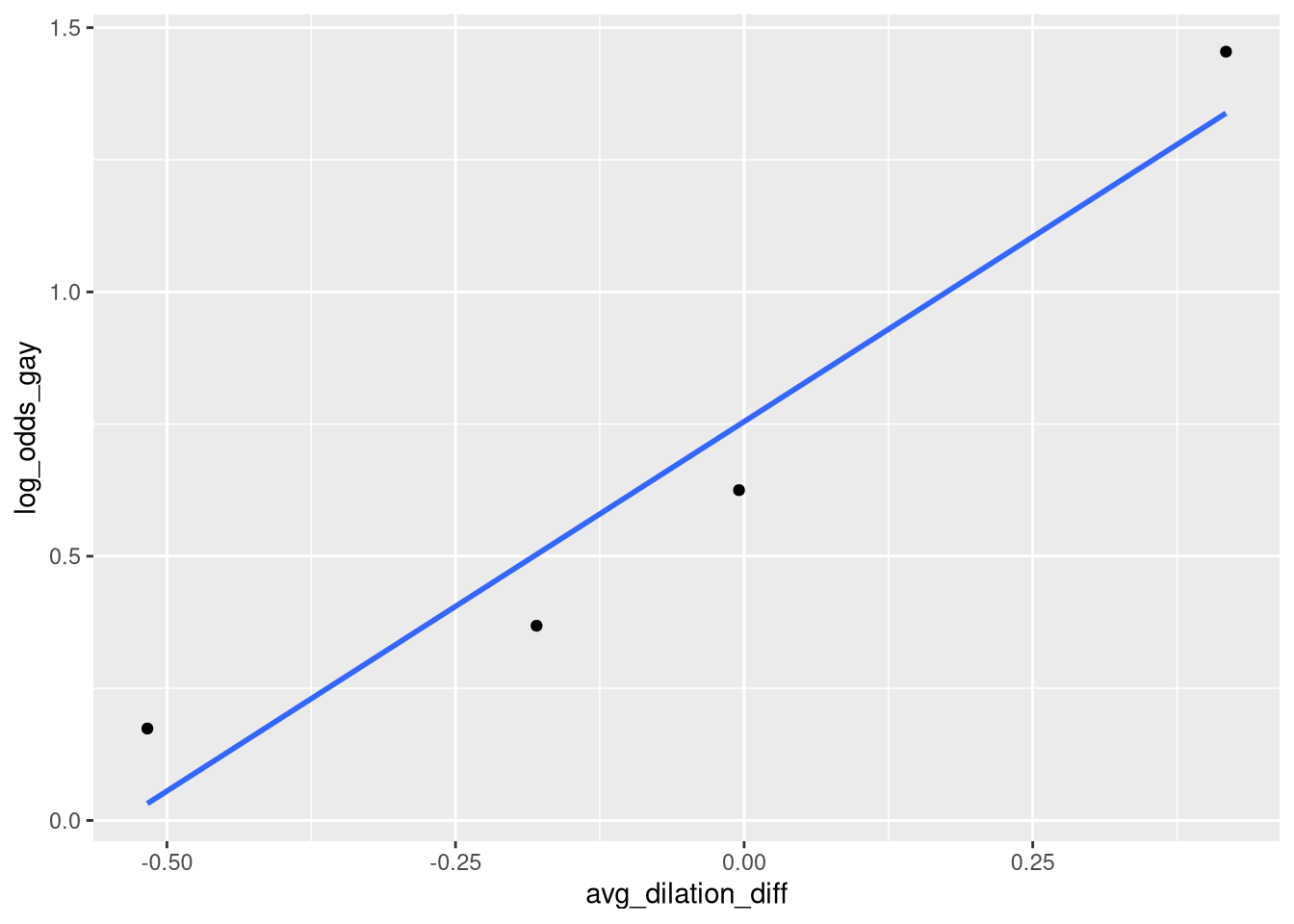

It is worth pointing out that while Figure 10.2, Figure 10.3, and Figure 10.4 all have log-odds on the y-axis, and lines of ‘best fit’ drawn in them, none of these plots visualize the predictions of a logistic regression model. These plots all represent linear regression models fit to the log-odds of “success”; this is useful for exploratory purposes, but not suitable for a final analysis.

To obtain an unbiased estimate of the log-odds of “success”, we need to fit a multiple logistic regression model to the raw “success” and “failure” observations. This is only slightly more difficult that fitting a “simple” logistic regression model; all we are required to do differently is literally add a second explanatory variable to the model formula in R!

One bit of data wrangling is helpful first; replacing the 0’s representing female participants with the word “Female”, and replacing the 1’s representing male participants with the word “Female”

Eyes <- Eyes |>
  mutate(Sex = recode(SexMale, `0`="Female", `1`="Male"))

gay_dilation_model <- glm(Gay ~ DilateDiff + Sex, data = Eyes,
                          family = binomial
                          )
summary(gay_dilation_model)$coefficients

             Estimate Std. Error   z value     Pr(>|z|)
(Intercept) -1.265639  0.3820190 -3.313025 9.229257e-04
DilateDiff   3.290778  0.8180317  4.022800 5.751032e-05
SexMale      1.289656  0.4952921  2.603830 9.218853e-03

Figure 10.5 shows the predictions of the fitted model in both the probability and logit forms. We can reproduce these figures using the same techniques from Chapter 9.1:

1. Create a “reference grid”, representing every combination of the explanatory variables we wish to obtain a prediction for
2. Use the broom::augment() function to obtain a prediction for every value in the grid
3. Plot these predictions using geom_line()

The only added complication is that here, we must use the expand.grid() function to create our “reference grid”, since we care about obtaining a prediction for many, closely spaced values of the DilateDiff variable, for both male and female participants.

ref_grid <- expand.grid(DilateDiff = seq(from = min(Eyes$DilateDiff),
                                         to = max(Eyes$DilateDiff),
                                         by = .01
                                         ),
                        Sex = c("Female", "Male")
                        )

head(ref_grid)

tail(ref_grid)

With our reference grid created, we can move on to step 2 and 3 to re-created Panel B:

library(broom)

predicted_odds <- augment(gay_dilation_model, newdata = ref_grid)
predicted_odds

ggplot(data = predicted_odds, aes(x=DilateDiff, y=.fitted, color=Sex)) +
  geom_line()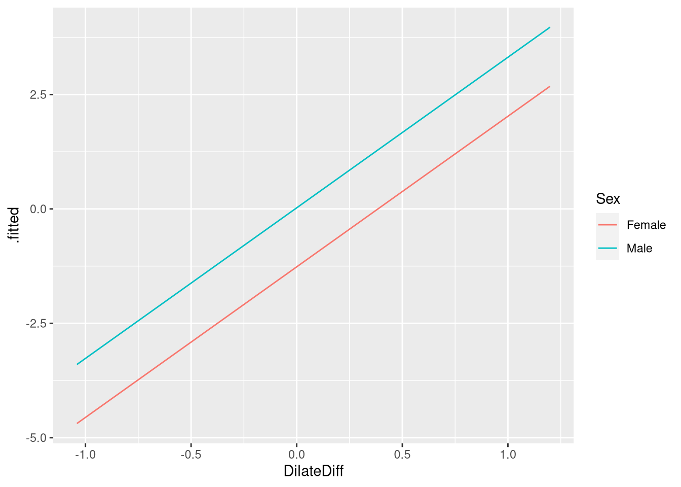

Panel A can be re-created by asking the augment() function to return it’s predictions on the "response" scale (i.e., with the log-odds squashed between 0 and 1, using the logistic transformation):

predicted_prob <- augment(gay_dilation_model, newdata = ref_grid,
                          type.predict = "response"
                          )
predicted_prob

ggplot(data = predicted_prob, aes(x=DilateDiff, y=.fitted, color=Sex)) +
  geom_line()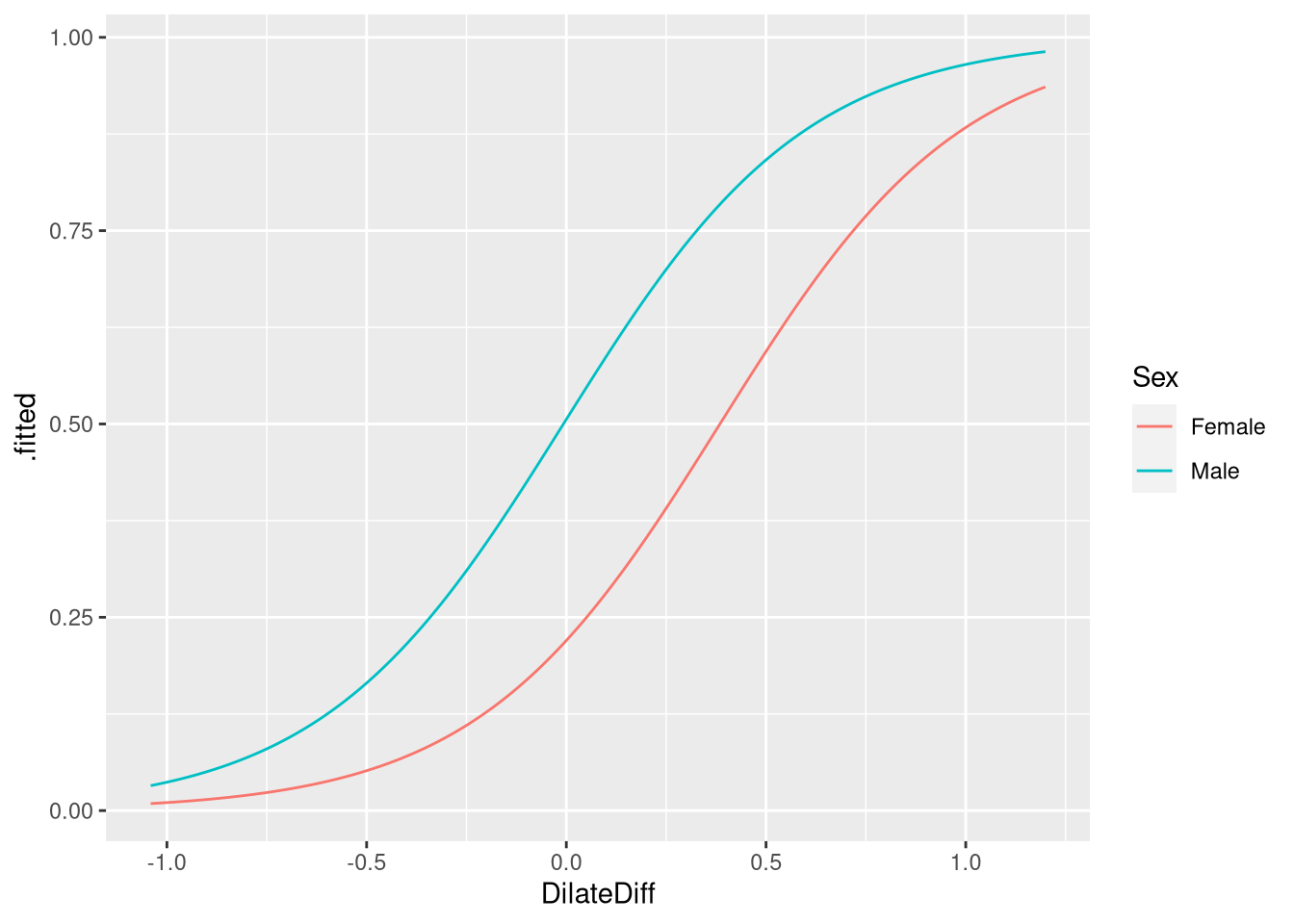

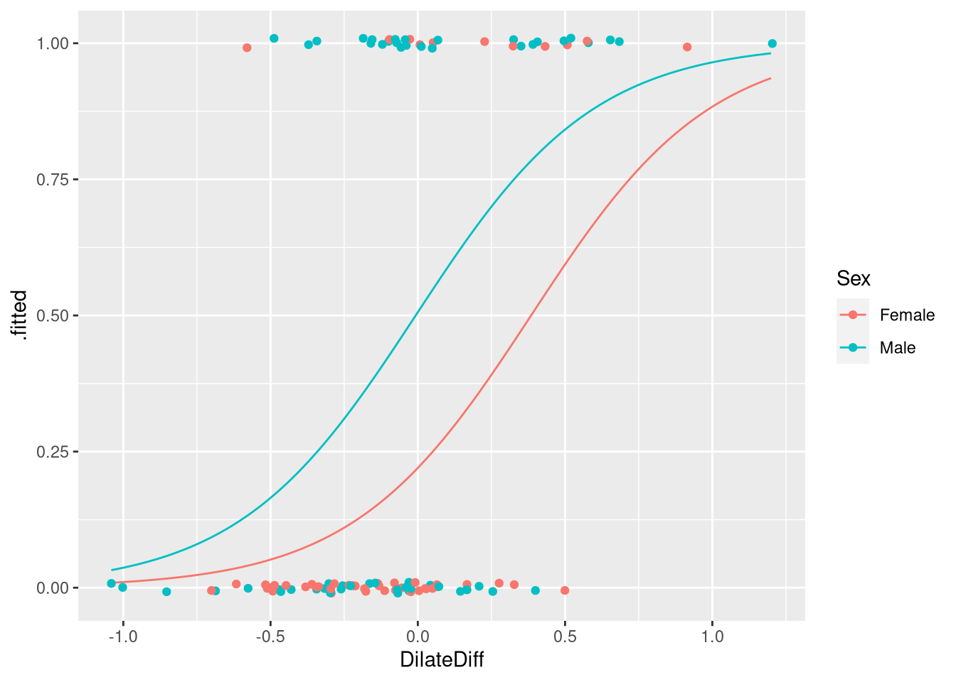
We could even add the raw data to this plot, since the raw data were measured on the 0/1 scale

ggplot(data = predicted_prob, aes(x=DilateDiff, y=.fitted, color=Sex)) +
  geom_line() +
  geom_jitter(data = Eyes,
              mapping = aes(y = Gay),
              height = .01
              )

10.2.2 Example 10.2: Medical school admissions

---

1. Ironically, the Kinsey scale was originally developed as a way of understanding sexual preferences without explicitly categorizing people as exclusively heterosexual, homosexual or bisexual!