Chapter 4 Tools & Advice for Instructors
4.1 Best Practices
4.1.2 Naming Objects
There are relatively few constraints to naming objects in R compared to other statistical software packages. We make several recommendations here for good naming practices.
The “naming conventions” of a particular programming language refer to the formatting guidelines for object names. There are no agreed-upon naming conventions in R, but a good overview can be found here. In general, the best advice is to pick a convention that appeals to you and use it consistently. We recommend the “underscore_separated” scheme. Because period separation can sometimes refer to a different process in R, we do not recommend using the “period.separated” scheme.
Regardless of the convention, it is also important to choose object names that are informative. That is, someone with little knowledge of the script, including some future version of yourself, should be able to get a general idea of what data an object contains based on the name. For instance, simply naming all versions of a data frame data, data_2, data_3, etc., is not informative because it is unclear what changes have been made between versions.
4.1.3 Scripting
More than just a collection of commands, the script is an excellent tool for both both reproducibility and documentation of an analysis. It is therefore worthwhile to teach students good habits for writing scripts.
First and foremost, scripts should include all of the commands that you need to conduct an analysis, and none of the commands that you don’t. That is, you should be able to run all of the lines in a script in order and get the same result each time (with the obvious exception of things like drawing random samples). To that end, all the commands necessary for an analysis should be in the proper sequence, and deny commands that are not necessary for the analysis but kept for posterity should be “commented out” by adding the # symbol at the start of the line.
Second, scripts should be well-documented. Recall that you can add comments to any line by preceding the comment with the # symbol. Comments are an efficient way to explain to someone unfamiliar with the script what the intention is for each section of code. Ample documentation is not only a good programming habit to teach your students, it will also likely be very useful in helping you decipher their code.
4.1.4 Formatting Requirements for Assignments
We encourage you to give your students clear formatting guidelines for assignments that require a significant amount of R programming to complete. The specific requirements that you decide on should be based on (1) the extent to which you want them to leave the class with generalizeable programming skills, and (2) the amount of detail that you would like from your students in terms of their code.
Asking students to print the contents of their console will allow you to see all of the commands that they ran, the order in which they ran them, as well as the output and any error messages, but it will be quite a lot of information for you to sort through yourself. At the other extreme, asking for only the formatted results in a Word document makes it difficult to judge the quality of their code, which may be a primary goal of the assignment. A nice compromise is to ask for an electronic version of their script with all the necessary commands so that you can reproduce their results. This can either act as the main document or as a supplement to a formatted report.
It has also become increasingly popular for instructors to provide students with prepared R Markdown (.Rmd) files with fill-in-the-blank style prompts for students to enter their code. This produces a nicely formatted document with their code and output, which may be easier for you administratively. However, this can also obscure the coding process for students and limit their independence. For this reason, we recommend against using prepared R Markdown files, and encourage you to teach students how to create and maintain their own scripts instead.
4.2 Error Messages
All messages printed to the console in red text are meant to get your attention, but they differ in urgency. A message with Error printed at the beginning means that there was a problem that prevented the command from being evaluated, and you will not be able to run that command until you fix the problem. A message with Warning printed at the beginning means that the command was evaluated, but it might not have worked the way you intended, or R might have made some decision for you in order to execute the command. All other messages can generally be taken as updates on the status of your command.
If you receive an error message that is unclear, the best way to determine the cause is to Google it. A list of the most common errors is provided here for convenience.
There is no output from a command, and there is a + in the console instead of a >.
The user has not completed the command, most likely by forgetting to close a quotation (or being inconsistent with the use of single vs. double quotations) or a set of parentheses. You can either add the end quotation or parenthesis if it is the final character, or press the escape button and start again.
Error: unexpected ')' in '___'
The user has included one too many end parentheses.
Error: Object '___' not found
The user has tried to call an object that is not in the environment. This may be because there is a typo in the name of the object, or because the object was never assigned to a label with the <- operator.
Error in ___ : non-numeric argument to binary operator
The user is most likely trying to conduct a mathematical operation on data that is of a non-numeric class, such as character or factor. If the data should be numeric, try overwriting it with as.numeric().
Error in ___(x) : could not find function '___'
The user is attempting to use a function that is not currently available in R, either because there is a typo in the name of the function or because the function’s package has not been loaded in this session.
Error in ___ : cannot open the connection
The user is attempting to read or write a file at a location on the hard drive that does not exist, likely due to a typo in the file path or file name.
Error in ___ : undefined columns selected** or **Error in ___: subscript out of bounds
The user is attempting to index an area of an object that does not exist, for instance, the ninth column of a seven-column data frame.
Error: unexpected symbol in '___'
R cannot interpret part of the command, likely because the user has forgotten a comma between function arguments.
4.3 Data Sets
This section includes an overview of some selected data sets that may be useful for in-class demonstrations or assignments. The first section includes data sets that are “built-in” as part of the base R datasets package, whereas the remaining sections review data sets from other selected packages that need to be installed. Of course, this list is non-exhaustive. The packages used here have more data sets than those we have chosen to highlight, and there are many more interesting data sets in other packages we have not highlighted. So, feel free to explore more options.
To see all of the data sets available from all loaded packages, including those are built-in with base R, enter the following command:
data()You should see a list of all the available data sets with a brief summary of each, separated by the package they belong to. To see a list of datsets in all installed packages (loaded or not), run the command data(package = .packages(all.available = TRUE)).
4.3.1 How to Handle NA Values
Most of the data sets below include at least some missing data, marked as NA, in at least one variable. Because, as you know, missing data is a problem that is sure to appear in the wild for students who continue on a research path, you may choose to teach students how to handle NA values themselves. Alternatively, you may choose to remove NA values on your own for simplicity, either by removing them from the data set beforehand (in which case the data would need to be saved as a .CSV file for the students to read in later), or providing students with code to run before beginning the assignment. Regardless, this section reviews how to handle NA values.
As mentioned previously, NA values can be identified with the is.na() function. For instance, imagine that we want to identify the missing quantitative SAT scores in the sat.act data set. We can first call is.na() on the variable to create a logical vector marking each NA as TRUE:
is.na(sat.act$SATQ)## [1] FALSE FALSE FALSE FALSE FALSE FALSE FALSE FALSE FALSE FALSE FALSE
## [12] FALSE FALSE FALSE FALSE FALSE FALSE FALSE FALSE FALSE FALSE FALSE
## [23] FALSE FALSE FALSE FALSE FALSE FALSE FALSE FALSE FALSE FALSE FALSE
## [34] FALSE FALSE FALSE FALSE FALSE FALSE FALSE FALSE FALSE FALSE FALSE
## [45] FALSE FALSE FALSE FALSE FALSE FALSE FALSE FALSE FALSE FALSE FALSE
## [56] FALSE FALSE FALSE FALSE FALSE FALSE FALSE FALSE FALSE FALSE FALSE
## [67] FALSE FALSE FALSE FALSE FALSE FALSE FALSE FALSE FALSE FALSE FALSE
## [78] FALSE FALSE FALSE FALSE FALSE FALSE FALSE FALSE FALSE FALSE FALSE
## [89] FALSE FALSE FALSE FALSE FALSE FALSE FALSE FALSE FALSE FALSE FALSE
## [100] FALSE FALSE FALSE FALSE FALSE FALSE FALSE FALSE FALSE FALSE FALSE
## [111] FALSE FALSE FALSE FALSE FALSE FALSE FALSE FALSE FALSE FALSE FALSE
## [122] FALSE FALSE FALSE FALSE FALSE FALSE FALSE FALSE TRUE FALSE FALSE
## [133] FALSE FALSE FALSE FALSE FALSE FALSE FALSE FALSE FALSE FALSE FALSE
## [144] FALSE FALSE FALSE FALSE FALSE FALSE FALSE FALSE FALSE FALSE FALSE
## [155] FALSE FALSE FALSE FALSE FALSE FALSE FALSE FALSE FALSE FALSE FALSE
## [166] FALSE FALSE FALSE FALSE FALSE FALSE FALSE FALSE FALSE FALSE FALSE
## [177] FALSE FALSE FALSE FALSE FALSE FALSE FALSE FALSE FALSE FALSE FALSE
## [188] FALSE FALSE FALSE FALSE FALSE FALSE FALSE FALSE FALSE TRUE FALSE
## [199] FALSE FALSE FALSE FALSE FALSE FALSE FALSE FALSE FALSE FALSE FALSE
## [210] FALSE FALSE FALSE FALSE FALSE FALSE FALSE FALSE FALSE FALSE FALSE
## [221] FALSE FALSE FALSE FALSE FALSE FALSE FALSE FALSE FALSE FALSE FALSE
## [232] FALSE FALSE FALSE FALSE FALSE FALSE FALSE FALSE FALSE FALSE FALSE
## [243] FALSE FALSE FALSE FALSE FALSE TRUE FALSE FALSE FALSE FALSE FALSE
## [254] FALSE FALSE FALSE FALSE FALSE FALSE FALSE FALSE FALSE FALSE FALSE
## [265] FALSE FALSE FALSE FALSE FALSE FALSE FALSE FALSE FALSE FALSE FALSE
## [276] FALSE FALSE FALSE FALSE FALSE FALSE FALSE FALSE FALSE FALSE FALSE
## [287] FALSE FALSE FALSE FALSE FALSE FALSE FALSE FALSE FALSE FALSE FALSE
## [298] FALSE FALSE FALSE FALSE FALSE FALSE FALSE FALSE FALSE FALSE FALSE
## [309] FALSE FALSE FALSE FALSE FALSE FALSE FALSE FALSE FALSE FALSE FALSE
## [320] FALSE FALSE FALSE FALSE FALSE FALSE FALSE FALSE FALSE FALSE FALSE
## [331] FALSE FALSE FALSE FALSE FALSE FALSE FALSE FALSE FALSE FALSE FALSE
## [342] FALSE FALSE FALSE FALSE FALSE FALSE FALSE FALSE FALSE FALSE FALSE
## [353] FALSE FALSE FALSE FALSE FALSE FALSE FALSE FALSE FALSE FALSE FALSE
## [364] TRUE FALSE FALSE FALSE FALSE FALSE FALSE FALSE FALSE FALSE FALSE
## [375] FALSE TRUE FALSE FALSE FALSE FALSE FALSE FALSE FALSE FALSE FALSE
## [386] FALSE FALSE FALSE FALSE FALSE FALSE FALSE FALSE FALSE FALSE FALSE
## [397] FALSE FALSE FALSE FALSE FALSE FALSE FALSE FALSE FALSE FALSE FALSE
## [408] FALSE FALSE FALSE FALSE FALSE FALSE FALSE FALSE FALSE FALSE FALSE
## [419] TRUE FALSE FALSE FALSE FALSE FALSE FALSE FALSE FALSE FALSE FALSE
## [430] FALSE FALSE FALSE FALSE FALSE FALSE FALSE FALSE FALSE FALSE FALSE
## [441] FALSE FALSE FALSE FALSE FALSE FALSE FALSE FALSE FALSE FALSE FALSE
## [452] FALSE FALSE FALSE FALSE FALSE FALSE FALSE FALSE FALSE FALSE FALSE
## [463] FALSE FALSE FALSE FALSE FALSE FALSE FALSE FALSE FALSE FALSE FALSE
## [474] FALSE FALSE FALSE FALSE FALSE FALSE FALSE FALSE FALSE FALSE FALSE
## [485] FALSE FALSE FALSE FALSE FALSE FALSE FALSE FALSE FALSE FALSE FALSE
## [496] FALSE FALSE TRUE FALSE FALSE FALSE FALSE FALSE FALSE FALSE FALSE
## [507] FALSE FALSE FALSE FALSE FALSE FALSE FALSE FALSE TRUE FALSE FALSE
## [518] FALSE FALSE FALSE FALSE FALSE TRUE FALSE FALSE FALSE FALSE FALSE
## [529] FALSE FALSE FALSE FALSE FALSE FALSE FALSE FALSE FALSE FALSE FALSE
## [540] FALSE FALSE FALSE FALSE FALSE FALSE FALSE FALSE FALSE FALSE FALSE
## [551] FALSE FALSE FALSE FALSE FALSE FALSE FALSE FALSE FALSE FALSE FALSE
## [562] FALSE FALSE FALSE FALSE FALSE FALSE FALSE FALSE FALSE FALSE FALSE
## [573] FALSE FALSE FALSE FALSE FALSE FALSE FALSE FALSE TRUE FALSE FALSE
## [584] FALSE FALSE FALSE FALSE FALSE FALSE FALSE FALSE FALSE FALSE FALSE
## [595] FALSE FALSE FALSE FALSE FALSE FALSE FALSE FALSE FALSE FALSE FALSE
## [606] FALSE FALSE FALSE FALSE FALSE FALSE FALSE FALSE FALSE FALSE FALSE
## [617] FALSE FALSE FALSE FALSE FALSE FALSE FALSE FALSE FALSE FALSE FALSE
## [628] FALSE FALSE FALSE FALSE FALSE FALSE FALSE FALSE FALSE FALSE FALSE
## [639] TRUE FALSE FALSE FALSE FALSE FALSE FALSE FALSE FALSE FALSE FALSE
## [650] FALSE FALSE FALSE FALSE FALSE FALSE TRUE FALSE FALSE FALSE FALSE
## [661] FALSE FALSE FALSE FALSE FALSE FALSE FALSE FALSE FALSE FALSE FALSE
## [672] FALSE FALSE TRUE FALSE FALSE FALSE FALSE FALSE FALSE FALSE FALSE
## [683] FALSE FALSE FALSE FALSE FALSE FALSE FALSE FALSE FALSE FALSE FALSE
## [694] FALSE FALSE FALSE FALSE FALSE FALSE FALSEThis logical vector can then be used to index the variable in question:
sat.act[is.na(sat.act$SATQ), 'SATQ']## [1] NA NA NA NA NA NA NA NA NA NA NA NA NAThe previous command returns the NA values because we have asked R to show us all of the values in sat.act$SATQ variable that are coded as NA. However, we are often more interested in the values that are NOT missing than those that are. To find the non-missing values, we can reverse the logical vector by adding the negation operator, !, to the beginning of the call to is.na():
sat.act[!is.na(sat.act$SATQ), 'SATQ']## [1] 500 500 470 520 550 640 500 560 600 800 710 600 600 725 630 590 650
## [18] 620 580 680 450 500 700 600 540 650 700 385 450 500 500 710 710 570
## [35] 580 600 600 570 540 690 610 610 700 610 740 540 650 600 440 690 780
## [52] 600 590 760 740 700 650 640 450 760 700 750 650 760 550 680 530 610
## [69] 600 550 450 740 530 750 700 565 590 590 375 550 500 500 760 580 590
## [86] 700 530 550 700 250 720 690 700 760 600 720 600 729 600 660 650 750
## [103] 660 680 700 610 650 550 710 480 740 720 630 560 700 700 500 660 500
## [120] 500 550 650 800 400 600 730 560 700 500 500 500 570 400 790 600 600
## [137] 620 700 720 680 610 690 770 770 550 530 720 320 800 800 600 800 700
## [154] 700 745 500 630 465 500 800 350 600 650 760 720 700 750 695 680 670
## [171] 540 500 500 800 680 640 600 680 600 650 580 400 750 678 530 600 675
## [188] 630 560 575 650 500 350 700 610 600 650 600 678 720 660 650 660 450
## [205] 670 620 480 500 555 800 710 630 770 710 600 560 550 350 450 460 700
## [222] 540 680 620 650 620 580 660 600 430 580 670 480 600 650 500 490 640
## [239] 570 680 720 500 660 600 570 650 550 200 690 460 525 675 700 700 650
## [256] 500 570 600 430 540 300 500 700 760 770 600 500 500 700 700 475 400
## [273] 750 600 650 480 520 720 300 780 520 400 550 450 680 800 725 540 690
## [290] 730 640 700 540 540 610 640 650 420 600 500 480 640 770 450 740 510
## [307] 650 600 700 700 750 450 450 600 750 650 300 700 750 540 300 600 480
## [324] 650 420 730 790 620 350 500 650 300 700 660 540 520 742 400 500 800
## [341] 570 690 680 500 640 700 600 650 520 540 609 800 690 780 640 580 750
## [358] 770 680 500 450 680 600 660 450 230 570 580 600 500 530 710 500 730
## [375] 450 550 760 450 740 770 690 540 650 300 440 420 640 690 400 710 500
## [392] 650 475 730 490 630 635 550 780 450 600 350 520 670 450 500 550 620
## [409] 550 600 740 620 670 560 710 700 480 800 760 650 550 720 650 700 660
## [426] 700 710 650 400 420 770 600 490 400 510 550 480 670 500 750 780 670
## [443] 640 710 750 650 300 700 720 600 600 590 650 500 650 680 400 480 400
## [460] 750 700 590 654 630 600 600 600 680 450 620 590 440 450 720 470 600
## [477] 700 640 500 530 640 799 800 600 800 600 550 600 450 750 560 590 500
## [494] 730 600 430 480 400 500 400 333 450 460 450 700 750 765 500 610 450
## [511] 450 500 600 600 600 670 620 660 700 600 620 680 677 640 596 660 530
## [528] 710 780 710 650 590 680 700 600 500 420 410 650 550 440 600 500 300
## [545] 530 600 400 730 610 600 720 780 490 700 680 400 800 740 760 720 720
## [562] 770 670 620 720 730 690 720 710 700 680 600 740 640 670 800 740 660
## [579] 800 400 640 710 680 680 700 640 690 720 510 690 770 640 500 590 640
## [596] 670 650 600 660 670 500 690 350 600 650 750 300 795 700 600 690 600
## [613] 650 600 710 690 500 700 740 430 684 610 750 430 780 770 600 550 760
## [630] 680 400 800 720 700 800 800 750 670 530 750 620 500 500 530 740 300
## [647] 670 700 690 800 750 500 580 700 600 540 690 600 520 500 720 600 700
## [664] 620 790 700 550 600 410 710 600 760 490 600 500 680 600 690 610 700
## [681] 660 680 500 630 630 780 600Now we’ve asked R to show us all of the values in the sat.act$SATQ variable that are NOT coded as NA.
To index the entire sat.act data frame so that all columns are returned, not just the quantitative SAT scores, use bracket notation without specifying any columns:
sat.act[!is.na(sat.act$SATQ), ]## gender education age ACT SATV SATQ SAT_diff
## 29442 2 3 19 24 500 500 0
## 29457 2 3 23 35 600 500 100
## 29498 2 3 20 21 480 470 10
## 29503 1 4 27 26 550 520 30
## 29504 1 2 33 31 600 550 50
## 29518 1 5 26 28 640 640 0Now we have the full sat.act data set, but only those rows where the quantitative SAT score is not NA. To be complete, we recommend saving this subset as a new object:
sat.act_noNA <- sat.act[!is.na(sat.act$SATQ), ]Note that you can also overwrite NA values, in cases where it is methodologically appropriate. For instance, perhaps you know that the students with missing quantitative SAT scores are treated as having a score of 0. You could replace the NA values with 0 as follows:
# First save a new version of the data
sat.act_NA0 <- sat.act

# Recode NA values as 0 in new version
sat.act_NA0[is.na(sat.act$SATQ), 'SATQ'] <- 0
Now all missing quantitative SAT scores will be treated as a 0 in future mathematical operations, using this new version of the data. Importantly, the original data frame is also preserved.
4.3.2 Built-In
There are several small data sets included in base R that are useful for quick demos. Since they are part of base R, it is not necessary to load these packages; just type and enter their name in the console to view them.
Note that the descriptions and summary statistics shown for each dataset were computed using the skim() function from the skimr pacakge.
iris
The iris data set gives the lengths and widths of the sepals and petals of 50 irises from each of three different species:
## Skim summary statistics
##  n obs: 150
##  n variables: 5
##
## -- Variable type:factor -------------------------------------
##  variable missing   n n_unique                       top_counts
##   Species       0 150        3 set: 50, ver: 50, vir: 50, NA: 0
##
## -- Variable type:numeric ------------------------------------
##      variable missing   n mean   sd     hist
##  Petal.Length       0 150 3.76 1.77 ▇▁▁▂▅▅▃▁
##   Petal.Width       0 150 1.2  0.76 ▇▁▁▅▃▃▂▂
##  Sepal.Length       0 150 5.84 0.83 ▂▇▅▇▆▅▂▂
##   Sepal.Width       0 150 3.06 0.44 ▁▂▅▇▃▂▁▁
warpbreaks
The warpbreaks data set gives the number of breaks in each of 54 looms of yarn, varied across two types of wool and three levels of tension:
## Skim summary statistics
##  n obs: 54
##  n variables: 3
##
## -- Variable type:factor -------------------------------------
##  variable missing  n n_unique                 top_counts
##   tension       0 54        3 L: 18, M: 18, H: 18, NA: 0
##      wool       0 54        2        A: 27, B: 27, NA: 0
##
## -- Variable type:numeric ------------------------------------
##  variable missing  n  mean   sd     hist
##    breaks       0 54 28.15 13.2 ▆▇▇▂▂▂▁▁
mtcars
The mtcars data set gives a range of numeric and categorical measurements of 32 cars, including MPG, number of cylinders, horsepower, weight, and transmission type:
## Skim summary statistics
##  n obs: 32
##  n variables: 11
##
## -- Variable type:numeric ------------------------------------
##  variable missing  n   mean     sd     hist
##        am       0 32   0.41   0.5  ▇▁▁▁▁▁▁▆
##      carb       0 32   2.81   1.62 ▆▇▂▇▁▁▁▁
##       cyl       0 32   6.19   1.79 ▆▁▁▃▁▁▁▇
##      disp       0 32 230.72 123.94 ▇▆▁▂▅▃▁▂
##      drat       0 32   3.6    0.53 ▃▇▁▅▇▂▁▁
##      gear       0 32   3.69   0.74 ▇▁▁▆▁▁▁▂
##        hp       0 32 146.69  68.56 ▃▇▃▅▂▃▁▁
##       mpg       0 32  20.09   6.03 ▃▇▇▇▃▂▂▂
##      qsec       0 32  17.85   1.79 ▃▂▇▆▃▃▁▁
##        vs       0 32   0.44   0.5  ▇▁▁▁▁▁▁▆
##        wt       0 32   3.22   0.98 ▃▃▃▇▆▁▁▂
ToothGrowth
The ToothGrowth data set gives the tooth lengths of 60 guinea pigs, varied across three vitamin C dosage levels and two dosage delivery methods:
## Skim summary statistics
##  n obs: 60
##  n variables: 3
##
## -- Variable type:factor -------------------------------------
##  variable missing  n n_unique            top_counts
##      supp       0 60        2 OJ: 30, VC: 30, NA: 0
##
## -- Variable type:numeric ------------------------------------
##  variable missing  n  mean   sd     hist
##      dose       0 60  1.17 0.63 ▇▁▇▁▁▁▁▇
##       len       0 60 18.81 7.65 ▃▅▃▅▃▇▂▂
4.3.3 FiveThirtyEight
The fivethirtyeight package includes data sets used for articles written on Nate Silver’s website for data geeks, FiveThirtyEight. From an instructional standpoint, these data sets are useful not only for being particularly engaging but because there is a published article associated with each one.
To make the data sets available, install and load the fivethirtyeight package:
install.packages('fivethirtyeight')
library(fivethirtyeight)
bechdel
The bechdel data set is a great all-purpose data set with both within- and between-subject continuous and categorical variables. Based on the Bechdel Test for female representation in film, this data set includes 1,794 movies from 1970-2013 along with their test outcome, budget, and gross profits:
## Skim summary statistics
##  n obs: 1794
##  n variables: 15
##
## -- Variable type:character ----------------------------------
##  variable missing    n min max empty n_unique
##    binary       0 1794   4   4     0        2
##      code       0 1794   8   8     0       85
##      imdb       0 1794   8  10     0     1794
##      test       0 1794   2  16     0       10
##     title       0 1794   1  83     0     1768
##
## -- Variable type:factor -------------------------------------
##    variable missing    n n_unique                            top_counts
##  clean_test       0 1794        5 ok: 803, not: 514, men: 194, dub: 142
##
## -- Variable type:integer ------------------------------------
##     variable missing    n       mean      sd     hist
##       budget       0 1794    4.5e+07 4.8e+07 ▇▂▁▁▁▁▁▁
##  budget_2013       0 1794    5.5e+07 5.5e+07 ▇▃▁▁▁▁▁▁
##  decade_code     179 1794    1.94    0.69    ▅▁▁▇▁▁▁▃
##  period_code     179 1794    2.42    1.19    ▇▇▁▆▁▅▁▂
##         year       0 1794 2002.55    8.98    ▁▁▁▁▂▅▅▇
##
## -- Variable type:numeric ------------------------------------
##       variable missing    n        mean          sd     hist
##       domgross      17 1794     6.9e+07 8e+07       ▇▂▁▁▁▁▁▁
##  domgross_2013      18 1794     9.5e+07     1.3e+08 ▇▁▁▁▁▁▁▁
##       intgross      11 1794     1.5e+08     2.1e+08 ▇▁▁▁▁▁▁▁
##  intgross_2013      11 1794 2e+08           2.8e+08 ▇▁▁▁▁▁▁▁
fandango
The fandango data set shows ratings from 146 movies across the Fandango, IMDB, Rotten Tomatoes, and Metacritic websites. It is particularly useful for demonstrating correlation:
## Skim summary statistics
##  n obs: 146
##  n variables: 23
##
## -- Variable type:character ----------------------------------
##  variable missing   n min max empty n_unique
##      film       0 146   3  63     0      146
##
## -- Variable type:integer ------------------------------------
##                    variable missing   n     mean       sd     hist
##              fandango_votes       0 146  3848.79  6357.78 ▇▂▁▁▁▁▁▁
##        imdb_user_vote_count       0 146 42846.21 67406.51 ▇▂▁▁▁▁▁▁
##                  metacritic       0 146    58.81    19.52 ▁▆▅▆▇▆▇▅
##  metacritic_user_vote_count       0 146   185.71   316.61 ▇▁▁▁▁▁▁▁
##              rottentomatoes       0 146    60.85    30.17 ▃▃▂▃▃▂▅▇
##         rottentomatoes_user       0 146    63.88    20.02 ▃▃▃▆▅▅▇▇
##
## -- Variable type:numeric ------------------------------------
##                    variable missing   n    mean   sd     hist
##         fandango_difference       0 146    0.24 0.15 ▃▇▁▆▇▁▇▃
##        fandango_ratingvalue       0 146    3.85 0.5  ▂▃▃▇▇▇▇▂
##              fandango_stars       0 146    4.09 0.54 ▂▃▁▆▁▇▁▂
##                        imdb       0 146    6.74 0.96 ▁▁▃▃▅▇▅▂
##                   imdb_norm       0 146    3.37 0.48 ▁▁▃▃▅▇▅▂
##             imdb_norm_round       0 146    3.38 0.5  ▁▂▁▅▇▁▅▁
##             metacritic_norm       0 146    2.94 0.98 ▁▆▅▆▇▆▇▅
##       metacritic_norm_round       0 146    2.97 0.99 ▁▆▅▆▇▆▇▅
##             metacritic_user       0 146    6.52 1.51 ▂▂▂▅▇▇▆▂
##         metacritic_user_nom       0 146    3.26 0.76 ▂▂▂▅▇▇▆▂
##  metacritic_user_norm_round       0 146    3.27 0.79 ▂▂▃▅▇▆▂▁
##                     rt_norm       0 146    3.04 1.51 ▃▃▂▃▃▂▅▇
##               rt_norm_round       0 146    3.07 1.51 ▅▃▁▃▂▂▂▇
##                rt_user_norm       0 146    3.19 1    ▃▃▃▆▅▅▇▇
##          rt_user_norm_round       0 146    3.23 1.01 ▁▃▂▆▅▅▇▇
##                        year       0 146 2014.88 0.32 ▁▁▁▁▁▁▁▇
comma_survey
The comma_survey data set has Likert ratings as well as demographic information collected from 1,129 respondents to a survey on the Oxford comma:
## Skim summary statistics
##  n obs: 1129
##  n variables: 13
##
## -- Variable type:character ----------------------------------
##              variable missing    n min max empty n_unique
##                gender      92 1129   4   6     0        2
##              location     102 1129   7  18     0        9
##  more_grammar_correct       0 1129  57  58     0        2
##       write_following      36 1129  76  77     0        2
##
## -- Variable type:factor -------------------------------------
##             variable missing    n n_unique
##                  age      92 1129        4
##            care_data      38 1129        4
##    care_oxford_comma      30 1129        4
##  care_proper_grammar      70 1129        5
##            education     103 1129        5
##     household_income     293 1129        5
##                              top_counts
##  45-: 290, > 6: 272, 30-: 254, 18-: 221
##  Not: 403, Som: 352, Not: 203, A l: 133
##  Som: 414, A l: 291, Not: 268, Not: 126
##     Ver: 688, Som: 333, NA: 70, Nei: 26
##   Bac: 344, Som: 295, Gra: 276, NA: 103
##   NA: 293, $50: 290, $10: 164, $25: 158
##
## -- Variable type:logical ------------------------------------
##              variable missing    n mean                      count
##  data_singular_plural      38 1129  0.5 FAL: 547, TRU: 544, NA: 38
##    heard_oxford_comma      30 1129  0.6 TRU: 655, FAL: 444, NA: 30
##
## -- Variable type:numeric ------------------------------------
##       variable missing    n    mean         sd     hist
##  respondent_id       0 1129 3.3e+09 1072966.47 ▇▃▇▇▆▂▁▂
avengers
The avengers data set includes the death and revival status for 173 Marvel comic book characters. It largely includes count and categorical data:
## Skim summary statistics
##  n obs: 173
##  n variables: 21
##
## -- Variable type:character ----------------------------------
##                     variable missing   n min max empty n_unique
##  full_reserve_avengers_intro      14 173   5   6     0       93
##                       gender       0 173   4   6     0        2
##                     honorary       0 173   4  12     0        4
##                   name_alias      10 173   4  35     0      162
##                        notes      98 173  21 255     0       71
##           probationary_intro     158 173   6   6     0       12
##                          url       0 173  36  67     0      173
##
## -- Variable type:integer ------------------------------------
##             variable missing   n    mean     sd     hist
##          appearances       0 173  414.05 677.99 ▇▁▁▁▁▁▁▁
##                 year       0 173 1988.45  30.37 ▂▁▁▁▂▂▃▇
##  years_since_joining       0 173   26.55  30.37 ▇▃▂▂▁▁▁▂
##
## -- Variable type:logical ------------------------------------
##  variable missing   n mean                     count
##   current       0 173 0.47   FAL: 91, TRU: 82, NA: 0
##    death1       0 173 0.4   FAL: 104, TRU: 69, NA: 0
##    death2     156 173 0.94  NA: 156, TRU: 16, FAL: 1
##    death3     171 173 1              NA: 171, TRU: 2
##    death4     172 173 1              NA: 172, TRU: 1
##    death5     172 173 1              NA: 172, TRU: 1
##   return1     104 173 0.67 NA: 104, TRU: 46, FAL: 23
##   return2     157 173 0.5    NA: 157, FAL: 8, TRU: 8
##   return3     171 173 0.5    NA: 171, FAL: 1, TRU: 1
##   return4     172 173 1              NA: 172, TRU: 1
##   return5     172 173 1              NA: 172, TRU: 1
bob_ross
The bob_ross data set is a great tool for demonstrating count data and tables. For each of 403 episodes, the data set marks the presence or absence of a series of possible elements in Bob’s painting. Useful combinations include tables of trees, lakes, and snowy mountains:
## Skim summary statistics
##  n obs: 403
##  n variables: 71
##
## -- Variable type:character ----------------------------------
##  variable missing   n min max empty n_unique
##   episode       0 403   6   6     0      403
##     title       0 403   8  27     0      401
##
## -- Variable type:integer ------------------------------------
##            variable missing   n   mean    sd     hist
##         apple_frame       0 403 0.0025 0.05  ▇▁▁▁▁▁▁▁
##     aurora_borealis       0 403 0.005  0.07  ▇▁▁▁▁▁▁▁
##                barn       0 403 0.042  0.2   ▇▁▁▁▁▁▁▁
##               beach       0 403 0.067  0.25  ▇▁▁▁▁▁▁▁
##                boat       0 403 0.005  0.07  ▇▁▁▁▁▁▁▁
##              bridge       0 403 0.017  0.13  ▇▁▁▁▁▁▁▁
##            building       0 403 0.0025 0.05  ▇▁▁▁▁▁▁▁
##              bushes       0 403 0.3    0.46  ▇▁▁▁▁▁▁▃
##               cabin       0 403 0.17   0.38  ▇▁▁▁▁▁▁▂
##              cactus       0 403 0.0099 0.099 ▇▁▁▁▁▁▁▁
##        circle_frame       0 403 0.005  0.07  ▇▁▁▁▁▁▁▁
##              cirrus       0 403 0.069  0.25  ▇▁▁▁▁▁▁▁
##               cliff       0 403 0.02   0.14  ▇▁▁▁▁▁▁▁
##              clouds       0 403 0.44   0.5   ▇▁▁▁▁▁▁▆
##             conifer       0 403 0.53   0.5   ▇▁▁▁▁▁▁▇
##             cumulus       0 403 0.21   0.41  ▇▁▁▁▁▁▁▂
##           deciduous       0 403 0.56   0.5   ▆▁▁▁▁▁▁▇
##         diane_andre       0 403 0.0025 0.05  ▇▁▁▁▁▁▁▁
##                dock       0 403 0.0025 0.05  ▇▁▁▁▁▁▁▁
##   double_oval_frame       0 403 0.0025 0.05  ▇▁▁▁▁▁▁▁
##                farm       0 403 0.0025 0.05  ▇▁▁▁▁▁▁▁
##               fence       0 403 0.06   0.24  ▇▁▁▁▁▁▁▁
##                fire       0 403 0.0025 0.05  ▇▁▁▁▁▁▁▁
##       florida_frame       0 403 0.0025 0.05  ▇▁▁▁▁▁▁▁
##             flowers       0 403 0.03   0.17  ▇▁▁▁▁▁▁▁
##                 fog       0 403 0.057  0.23  ▇▁▁▁▁▁▁▁
##              framed       0 403 0.13   0.34  ▇▁▁▁▁▁▁▁
##               grass       0 403 0.35   0.48  ▇▁▁▁▁▁▁▅
##               guest       0 403 0.055  0.23  ▇▁▁▁▁▁▁▁
##   half_circle_frame       0 403 0.0025 0.05  ▇▁▁▁▁▁▁▁
##     half_oval_frame       0 403 0.0025 0.05  ▇▁▁▁▁▁▁▁
##               hills       0 403 0.045  0.21  ▇▁▁▁▁▁▁▁
##                lake       0 403 0.35   0.48  ▇▁▁▁▁▁▁▅
##               lakes       0 403 0      0     ▁▁▁▇▁▁▁▁
##          lighthouse       0 403 0.0025 0.05  ▇▁▁▁▁▁▁▁
##                mill       0 403 0.005  0.07  ▇▁▁▁▁▁▁▁
##                moon       0 403 0.0074 0.086 ▇▁▁▁▁▁▁▁
##            mountain       0 403 0.4    0.49  ▇▁▁▁▁▁▁▅
##           mountains       0 403 0.25   0.43  ▇▁▁▁▁▁▁▂
##               night       0 403 0.027  0.16  ▇▁▁▁▁▁▁▁
##               ocean       0 403 0.089  0.29  ▇▁▁▁▁▁▁▁
##          oval_frame       0 403 0.094  0.29  ▇▁▁▁▁▁▁▁
##          palm_trees       0 403 0.022  0.15  ▇▁▁▁▁▁▁▁
##                path       0 403 0.12   0.33  ▇▁▁▁▁▁▁▁
##              person       0 403 0.0025 0.05  ▇▁▁▁▁▁▁▁
##            portrait       0 403 0.0074 0.086 ▇▁▁▁▁▁▁▁
##  rectangle_3d_frame       0 403 0.0025 0.05  ▇▁▁▁▁▁▁▁
##   rectangular_frame       0 403 0.0025 0.05  ▇▁▁▁▁▁▁▁
##               river       0 403 0.31   0.46  ▇▁▁▁▁▁▁▃
##               rocks       0 403 0.19   0.39  ▇▁▁▁▁▁▁▂
##      seashell_frame       0 403 0.0025 0.05  ▇▁▁▁▁▁▁▁
##                snow       0 403 0.19   0.39  ▇▁▁▁▁▁▁▂
##      snowy_mountain       0 403 0.27   0.44  ▇▁▁▁▁▁▁▃
##         split_frame       0 403 0.0025 0.05  ▇▁▁▁▁▁▁▁
##          steve_ross       0 403 0.027  0.16  ▇▁▁▁▁▁▁▁
##           structure       0 403 0.21   0.41  ▇▁▁▁▁▁▁▂
##                 sun       0 403 0.099  0.3   ▇▁▁▁▁▁▁▁
##          tomb_frame       0 403 0.0025 0.05  ▇▁▁▁▁▁▁▁
##                tree       0 403 0.9    0.31  ▁▁▁▁▁▁▁▇
##               trees       0 403 0.84   0.37  ▂▁▁▁▁▁▁▇
##        triple_frame       0 403 0.0025 0.05  ▇▁▁▁▁▁▁▁
##           waterfall       0 403 0.097  0.3   ▇▁▁▁▁▁▁▁
##               waves       0 403 0.084  0.28  ▇▁▁▁▁▁▁▁
##            windmill       0 403 0.0025 0.05  ▇▁▁▁▁▁▁▁
##        window_frame       0 403 0.0025 0.05  ▇▁▁▁▁▁▁▁
##              winter       0 403 0.17   0.38  ▇▁▁▁▁▁▁▂
##         wood_framed       0 403 0.0025 0.05  ▇▁▁▁▁▁▁▁
##
## -- Variable type:numeric ------------------------------------
##     variable missing   n mean   sd     hist
##  episode_num       0 403    7 3.75 ▇▇▃▇▃▇▃▇
##       season       0 403   16 8.96 ▇▇▇▇▆▇▇▇
4.3.4 psych
In addition to a range of new functions, the psych package includes data sets intended to demonstrate common statistical analyses for psychological research.
To make the data sets available, install and load the psych package:
install.packages('psych')
library(psych)
Tal.Or
The Tal.Or data set is from Study 2 of Tol-Or, Cohen, Tasfati, & Gunther (2010), which used an experimental manipulation to test the effects of media on the attitudes of 123 respondents, measured with Likert scales:
## Skim summary statistics
##  n obs: 123
##  n variables: 6
##
## -- Variable type:numeric ------------------------------------
##  variable missing   n  mean   sd     hist
##       age       0 123 24.63 5.8  ▇▇▁▁▁▁▁▁
##      cond       0 123  0.47 0.5  ▇▁▁▁▁▁▁▇
##    gender       0 123  1.65 0.48 ▅▁▁▁▁▁▁▇
##    import       0 123  4.2  1.74 ▃▃▅▇▁▇▇▃
##       pmi       0 123  5.6  1.32 ▁▁▁▂▂▆▆▇
##  reaction       0 123  3.48 1.55 ▇▆▇▆▅▆▃▂
affect
The affect data set consists of responses from 330 participants to state and trait mood scales given before and after viewing (1) a Frontline documentary about the liberation of a concentration camp, (2) the horror movie Halloween, (3) a National Geographic nature film about the Serengeti, or (4) the comedy movie Parenthood:
## Skim summary statistics
##  n obs: 330
##  n variables: 20
##
## -- Variable type:factor -------------------------------------
##  variable missing   n n_unique                top_counts
##     Study       0 330        2 fla: 170, map: 160, NA: 0
##
## -- Variable type:integer ------------------------------------
##  variable missing   n  mean    sd     hist
##      Film       0 330  2.52  1.13 ▇▁▇▁▁▇▁▇
##       MEQ     160 330 39.36 10.28 ▂▃▆▇▇▆▂▁
##
## -- Variable type:numeric ------------------------------------
##  variable missing   n  mean    sd     hist
##       BDI     170 330  0.31  0.28 ▇▆▅▁▁▁▁▁
##       EA1       0 330  9.19  7.11 ▇▆▃▅▃▂▂▁
##       EA2       0 330 11.01  6.85 ▇▇▅▇▆▃▂▁
##       ext       0 330 13.16  4.47 ▁▁▃▆▆▇▆▂
##       imp       0 330  4.29  1.97 ▃▅▆▆▇▃▅▂
##       lie       0 330  2.3   1.48 ▂▅▇▅▂▂▁▁
##       NA1       0 330  3.69  4.31 ▇▃▁▁▁▁▁▁
##       NA2       0 330  4.65  5.19 ▇▃▂▁▁▁▁▁
##      neur       0 330 10.22  5.04 ▂▅▆▇▇▃▂▁
##       PA1       0 330  8.89  6.79 ▇▇▆▅▃▂▁▁
##       PA2       0 330  8.98  6.43 ▇▆▅▆▅▁▁▁
##       soc       0 330  7.51  2.86 ▁▂▁▅▇▅▆▁
##    state1       0 330 40.83 10.76 ▃▆▇▅▃▁▁▁
##    state2     160 330 42.45 10.76 ▃▃▇▆▇▅▂▁
##       TA1       0 330 12.91  4.42 ▁▁▂▇▅▂▁▁
##       TA2       0 330 15.65  4.88 ▁▃▃▇▃▃▁▁
##  traitanx       0 330 39.52  9.77 ▃▅▇▅▂▂▁▁
epi
The epi data set includes responses to the Eysenck Personality Inventory from 3570 subjects:
## Skim summary statistics
##  n obs: 3570
##  n variables: 57
##
## -- Variable type:integer ------------------------------------
##  variable missing    n mean   sd     hist
##        V1     296 3570 1.28 0.45 ▇▁▁▁▁▁▁▃
##       V10      64 3570 1.86 0.35 ▁▁▁▁▁▁▁▇
##       V11      77 3570 1.3  0.46 ▇▁▁▁▁▁▁▃
##       V12      66 3570 1.2  0.4  ▇▁▁▁▁▁▁▂
##       V13      75 3570 1.44 0.5  ▇▁▁▁▁▁▁▆
##       V14      72 3570 1.25 0.43 ▇▁▁▁▁▁▁▂
##       V15      75 3570 1.79 0.41 ▂▁▁▁▁▁▁▇
##       V16      80 3570 1.51 0.5  ▇▁▁▁▁▁▁▇
##       V17      75 3570 1.22 0.42 ▇▁▁▁▁▁▁▂
##       V18      71 3570 1.17 0.37 ▇▁▁▁▁▁▁▂
##       V19      70 3570 1.21 0.41 ▇▁▁▁▁▁▁▂
##        V2      85 3570 1.47 0.5  ▇▁▁▁▁▁▁▇
##       V20      90 3570 1.23 0.42 ▇▁▁▁▁▁▁▂
##       V21      80 3570 1.35 0.48 ▇▁▁▁▁▁▁▅
##       V22     100 3570 1.43 0.49 ▇▁▁▁▁▁▁▆
##       V23      75 3570 1.62 0.49 ▅▁▁▁▁▁▁▇
##       V24      78 3570 1.74 0.44 ▃▁▁▁▁▁▁▇
##       V25      72 3570 1.31 0.46 ▇▁▁▁▁▁▁▃
##       V26      89 3570 1.7  0.46 ▃▁▁▁▁▁▁▇
##       V27     108 3570 1.38 0.49 ▇▁▁▁▁▁▁▅
##       V28      74 3570 1.35 0.48 ▇▁▁▁▁▁▁▅
##       V29      87 3570 1.67 0.47 ▅▁▁▁▁▁▁▇
##        V3      73 3570 1.45 0.5  ▇▁▁▁▁▁▁▇
##       V30      71 3570 1.18 0.39 ▇▁▁▁▁▁▁▂
##       V31      98 3570 1.35 0.48 ▇▁▁▁▁▁▁▅
##       V32      99 3570 1.72 0.45 ▃▁▁▁▁▁▁▇
##       V33      78 3570 1.63 0.48 ▅▁▁▁▁▁▁▇
##       V34      96 3570 1.4  0.49 ▇▁▁▁▁▁▁▆
##       V35      69 3570 1.86 0.35 ▂▁▁▁▁▁▁▇
##       V36     109 3570 1.72 0.45 ▃▁▁▁▁▁▁▇
##       V37      86 3570 1.63 0.48 ▅▁▁▁▁▁▁▇
##       V38      83 3570 1.76 0.43 ▂▁▁▁▁▁▁▇
##       V39      89 3570 1.46 0.5  ▇▁▁▁▁▁▁▇
##        V4      65 3570 1.57 0.5  ▆▁▁▁▁▁▁▇
##       V40      82 3570 1.47 0.5  ▇▁▁▁▁▁▁▇
##       V41      79 3570 1.71 0.45 ▃▁▁▁▁▁▁▇
##       V42      68 3570 1.2  0.4  ▇▁▁▁▁▁▁▂
##       V43      70 3570 1.81 0.39 ▂▁▁▁▁▁▁▇
##       V44      76 3570 1.9  0.3  ▁▁▁▁▁▁▁▇
##       V45      85 3570 1.79 0.41 ▂▁▁▁▁▁▁▇
##       V46      81 3570 1.54 0.5  ▇▁▁▁▁▁▁▇
##       V47      78 3570 1.76 0.43 ▂▁▁▁▁▁▁▇
##       V48      75 3570 1.18 0.38 ▇▁▁▁▁▁▁▂
##       V49      80 3570 1.17 0.38 ▇▁▁▁▁▁▁▂
##        V5      73 3570 1.2  0.4  ▇▁▁▁▁▁▁▂
##       V50      80 3570 1.46 0.5  ▇▁▁▁▁▁▁▇
##       V51      78 3570 1.76 0.43 ▂▁▁▁▁▁▁▇
##       V52      89 3570 1.65 0.48 ▅▁▁▁▁▁▁▇
##       V53      94 3570 1.58 0.49 ▆▁▁▁▁▁▁▇
##       V54      79 3570 1.42 0.49 ▇▁▁▁▁▁▁▆
##       V55      74 3570 1.52 0.5  ▇▁▁▁▁▁▁▇
##       V56      76 3570 1.57 0.49 ▆▁▁▁▁▁▁▇
##       V57      77 3570 1.8  0.4  ▂▁▁▁▁▁▁▇
##        V6      68 3570 1.43 0.5  ▇▁▁▁▁▁▁▆
##        V7      68 3570 1.41 0.49 ▇▁▁▁▁▁▁▆
##        V8      70 3570 1.65 0.48 ▅▁▁▁▁▁▁▇
##        V9      71 3570 1.46 0.5  ▇▁▁▁▁▁▁▇
sat.act
The sat.act data set includes self-reported SAT and ACT scores along with demographic information from 700 respondents, making it useful for within- or between-subject comparisons:
## Skim summary statistics
##  n obs: 700
##  n variables: 7
##
## -- Variable type:integer ------------------------------------
##   variable missing   n   mean     sd     hist
##        ACT       0 700  28.55   4.82 ▁▁▁▁▃▅▇▇
##        age       0 700  25.59   9.5  ▇▇▂▂▁▁▁▁
##  education       0 700   3.16   1.43 ▂▁▁▁▇▁▅▅
##     gender       0 700   1.65   0.48 ▅▁▁▁▁▁▁▇
##   SAT_diff      13 700   2.12  96.57 ▁▁▁▅▇▂▁▁
##       SATQ      13 700 610.22 115.64 ▁▁▁▅▃▇▇▅
##       SATV       0 700 612.23 112.9  ▁▁▁▃▃▇▅▃
4.3.5 Simulating your own Data Sets
If none of the available data sets satisfy your needs, or if you simply want to get creative, it is possible to simulate your own data set by drawing random samples from a distribution. This can be a great method of designing engaging data sets. It also ensures that you will have a nice “clean” data set, with no unwanted NA values, balanced or unbalanced designs as needed, and null and significant effects as desired.
To demonstrate how to simulate a numeric variable, the following code simulates income for 1,000 families from a population in which income is normally distributed around $50,000 with a standard deviation of $5,000:
sim_income <- rnorm(n=1000, mean=50000, sd=5000)
hist(sim_income)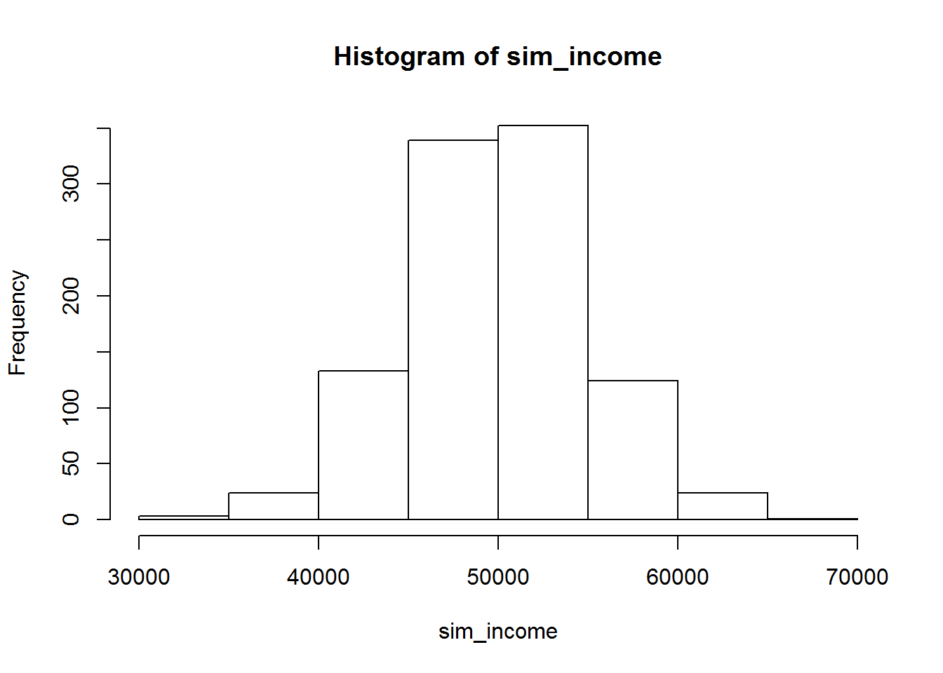
To demonstrate how to simulate a categorical variable, the following code simulates grades for 50 students in a pass/fail course in which there is a 50% chance of passing in the population:
sim_grades <- rbinom(n=50, size=1, prob=.5)
sim_grades <- factor(sim_grades, levels=0:1, labels=c('FAIL', 'PASS'))
barplot(table(sim_grades))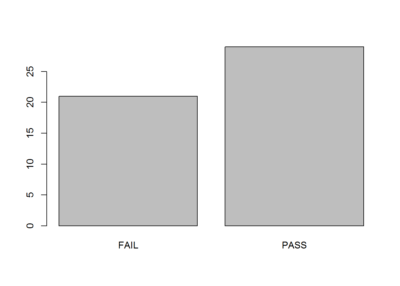
Other potentially useful “population” distributions include rbeta(), rbinom(), rchisq(), rexp(), rf(), rgamma(), rlogis(), rlnorm(), rpois(), rt(), and runif(). A full list can be found here. See the help documentation for each to see which parameter values can be specified.
Reproducibility
The R session information when compiling this book is shown below:
sessionInfo()## R version 3.5.1 (2018-07-02)
## Platform: x86_64-w64-mingw32/x64 (64-bit)
## Running under: Windows 7 x64 (build 7601) Service Pack 1
##
## Matrix products: default
##
## locale:
## [1] LC_COLLATE=English_United States.1252
## [2] LC_CTYPE=English_United States.1252
## [3] LC_MONETARY=English_United States.1252
## [4] LC_NUMERIC=C
## [5] LC_TIME=English_United States.1252
##
## attached base packages:
## [1] stats graphics grDevices utils datasets methods base
##
## other attached packages:
## [1] skimr_1.0.6 fivethirtyeight_0.4.0 psych_1.8.12
##
## loaded via a namespace (and not attached):
## [1] Rcpp_1.0.1 knitr_1.22 magrittr_1.5 tidyselect_0.2.5
## [5] mnormt_1.5-5 lattice_0.20-35 R6_2.4.0 rlang_0.3.4
## [9] highr_0.7 stringr_1.3.1 dplyr_0.8.1 tools_3.5.1
## [13] parallel_3.5.1 grid_3.5.1 packrat_0.4.9-3 nlme_3.1-137
## [17] xfun_0.6 cli_1.1.0 htmltools_0.3.6 yaml_2.2.0
## [21] digest_0.6.19 assertthat_0.2.1 tibble_2.1.1 crayon_1.3.4
## [25] bookdown_0.11 tidyr_0.8.3 purrr_0.3.2 codetools_0.2-15
## [29] glue_1.3.1 evaluate_0.14 rmarkdown_1.13 stringi_1.4.3
## [33] pillar_1.4.1 compiler_3.5.1 foreign_0.8-70 pkgconfig_2.0.2