• In the last lab we introduced some of dplyr's "Basic Verbs", i.e., functions for performing some of the most common tasks in data manipulation and analysis.
  • Removing rows –> filter()
  • Removing & renaming columns –> select() and rename()
  • Creating new columns –> mutate()
  • Summarizing measured variables –> summarise()
• Today we're going to look at how to combine these operations together to simplify your workflow, and some more 'advanced' features of the dplyr package.

Before we start, load dplyr and download the data. The marathon dataset holds the results of the 2009 Credit Union Cherry Blossom Ten Mile Run.

library(dplyr)
marathon <- read.csv("http://wjhopper.github.io//psych640-labs/data/marathon.csv")
str(marathon)

## 'data.frame':    14969 obs. of  11 variables:
##  $ place  : int  4554 3757 7625 7822 4355 2350 1404 672 5900 7483 ...
##  $ time   : num  108.4 95.8 130.9 133.9 100.5 ...
##  $ netTime: num  94.8 89.9 118.6 121.4 93.5 ...
##  $ age    : int  28 32 22 28 28 44 29 29 30 37 ...
##  $ gender : Factor w/ 2 levels "F","M": 2 2 1 1 2 1 2 2 2 1 ...
##  $ first  : Factor w/ 2941 levels "Aakar","Aaron",..: 1279 2085 1073 424 1087 1441 687 2444 1229 1383 ...
##  $ last   : Factor w/ 8755 levels "Aaronson","Abagon",..: 1 2 3 4 4 4 5 6 6 6 ...
##  $ city   : Factor w/ 1259 levels "Aberdeen","Abingdon",..: 1027 743 48 48 48 375 1172 1172 48 705 ...
##  $ state  : Factor w/ 51 levels "AE","AK","AL",..: 21 21 46 46 46 46 9 9 46 46 ...
##  $ country: Factor w/ 13 levels "AUS","CAN","ETH",..: 13 13 13 13 13 13 13 13 13 13 ...
##  $ div    : Factor w/ 14 levels "19-","20-24",..: 3 4 2 3 3 6 3 3 4 5 ...

Many serial steps of "tidying" our data are often necessary to perform any analysis of interest (e.g., first reshaping the data, then removing observations, etc.)

This "grunt work" is usually implemented using coding styles that make your scripts brittle and difficult to read

We'll examine the drawbacks of these styles by doing some prep work on the marathon dataset. Our job will be:

1. Move the ID variables to the left hand side
2. Make a variable showing the difference between time and netTime
3. Sort the data from first place to last place.

The goal of these examples is convince you that doing things "the dplyr way" is a better solution in most cases.

One way to make the results from each task feed into the next is to make a new variable after we finish each task, and use that variable as the input to the next function

marathon1 <- select(marathon, age:div, place:netTime)
marathon2 <- mutate(marathon1, waitTime = time - netTime)
marathon_sorted <- arrange(marathon2, place)

One drawback to this approach is that it promotes using uninformative variable names, like marathon1, because there aren't good single words to describe what has changed and most results are just intermediate, "one-off" data frames.

Additionally, it is prone to simple typos (missing the 1 on the end of marathon) and can use lots of memory in the long run by keeping copies of approximately identical data sets.

An alternative style is to re-assign the variable after each step: If you use marathon as the input to a function, overwrite the marathon variable with the output of that function.

marathon <- select(marathon, age:div, place:netTime)
marathon <- mutate(marathon, waitTime = time - netTime)
marathon <- arrange(marathon, place)

This is somewhat better semantically, but it also introduces ambiguity, especially in interactive situations. If you have a variable called marathon, what do you have? Is it the marathon variable after the select, or after the mutate or after the arrange?

When there are lots of steps, and you're running and re-running code, its easy to forget what you have and haven't done.

The intrepid coder who realizes the perils of constant object creation and overwriting variables may attempt to have it all. They want a single variable, assigned a single time, and they will get it by writing a single line of code!

marathon <- arrange(mutate(select(marathon, age:div, place:netTime),
                           waitTime = time - netTime),
                    place)

However the "one variable, assigned once" goal is achieved by sacrificing the readability of the function code.

Nesting many functions obscures which arguments belong to which functions, even when the arguments are broken down on different lines, and requires to write your functions "inside out".

Installing dplyr also installs another R package called magrittr, which provides an operator called a pipe.

A pipe sends the output of one function to another function as input. This allows you to chain functions together without nesting them, or assigning intermediate "one-off" variables.

The pipe operator is written %>%, and is loaded when dplyr is loaded. To get a feel for how it works, try these simple examples.

5 %>% sqrt() # Same as sqrt(5)

## [1] 2.236068

c(10,8,22) %>% mean() # Same as mean(c(10,8,22))

## [1] 13.33333

The output of the left-hand side function always becomes the value of the first unnamed argument to the right-hand side function. Let's look at this by changing the data from the mean example to include an NA. The mean function has 3 arguments: x (data), trim (percent to remove) and na.rm (include or remove missings).

c(10,NA,22) %>% mean(na.rm = TRUE) 

## [1] 16

Omitting the x argument would normally cause an error, but not here because its value is supplied via the %>% operator.

The vector c(10,NA,22) gets used as the value of the x argument (instead of trim) because x is the first argument not supplied in the argument list.

The first unnamed argument will receive its value through the pipe, regardless of serial position in the formal argument list.

Here TRUE gets piped to the na.rm argument because x and trim are supplied by name.

TRUE %>% mean(x=c(10,NA,22), trim=0)

## [1] 16

Below, TRUE gets piped to the x argument, since the numeric vector is not named. The piped value takes precedence, and the numeric vector gets used as the na.rm argument!

TRUE %>% mean(c(10,NA,22), trim=0)

## [1] 1

If you want to use the piped-in data as the value for several arguments, or reference it explicitly for clarities sake, you can use . inside the function call.

# cov (covariance) requires two args, x and y
c(19,38,14,20) %>% cov(x=., y=.) # piped data becomes x and y

## [1] 110.25

c(19,38,14,20) %>% cov(c(100,184,112,75), .) # piped data becomes y

## [1] 414.9167

c(19,38,14,20) %>% cov(y=.) # piped data becomes y, leaving no data for x

## Error in is.data.frame(x): argument "x" is missing, with no default

Pipes can simplify the flow of multi-step tasks that spans multiple functions by allowing you to write code that can be read left to right, top to bottom.

To see, lets write our marathon data tidying code using pipes. You can read the %>% operator as saying "then".

marathon <- read.csv("../data/marathon.csv") %>%
  select(age:div, place:netTime) %>%
  mutate(waitTime = time - netTime) %>%
  arrange(place)

We omit the data frame argument to select, mutate, and arrange because it is supplied from the previous functions output, via the pipe operator.

• A window function is a function that takes an input containing n elements and returns an output containing n elements
• The output of a window function depends on all the values in its input.
• Window functions which are particularly useful in conjunction with the mutate function.

The ntile() function ranks the data from each group into n clusters. This allows you to easily divide your data into as many bins as you like.

Here we'll create a variable identifying which netTime quintile each runner falls into, for males and females separately.

marathon <- marathon %>% group_by(gender) %>%
  mutate(quintile = ntile(netTime, 5))
select(marathon, gender:last, netTime, quintile)

## # A tibble: 14,969 x 5
## # Groups:   gender [2]
##   gender first           last        netTime quintile
##   <fct>  <fct>           <fct>         <dbl>    <int>
## 1 F      Lineth          Chepkurui      53.5        1
## 2 M      Ridouane        Harroufi       45.9        1
## 3 F      Belianesh Zemed Gebre          53.9        1
## 4 M      Feyisa          Liesa          46.0        1
## 5 F      Teyba           Naser          54.0        1
## 6 M      Silas           Sang           46.0        1
## 7 M      Karim           El Mabchour    46          1
## 8 F      Abebu           Gelan          54.4        1
## # ... with 1.496e+04 more rows

The percent_rank() function ranks each observation in your data according to what proportion of other observations in the group have a lower value.

marathon <- marathon %>%
  mutate(pBelow = percent_rank(netTime))
select(marathon, gender:last, netTime, pBelow)

## # A tibble: 14,969 x 5
## # Groups:   gender [2]
##   gender first           last        netTime   pBelow
##   <fct>  <fct>           <fct>         <dbl>    <dbl>
## 1 F      Lineth          Chepkurui      53.5 0       
## 2 M      Ridouane        Harroufi       45.9 0       
## 3 F      Belianesh Zemed Gebre          53.9 0.000120
## 4 M      Feyisa          Liesa          46.0 0.000150
## 5 F      Teyba           Naser          54.0 0.000240
## 6 M      Silas           Sang           46.0 0.000301
## 7 M      Karim           El Mabchour    46   0.000451
## 8 F      Abebu           Gelan          54.4 0.000361
## # ... with 1.496e+04 more rows

The lead() function takes a vector as input, and returns a vector where the elements have been moved to the left one position.

In other words, the first element in the output vector is second element of the input vector, the second element in the output vector is third element of the input vector, and so on.

lead(c(6,8,14,19,22))

## [1]  8 14 19 22 NA

The output vector is padded with an NA in the final position to make the input and output have the same number of elements.

You can think of lead as answering the question "What is the value of the element to my right?" for each element in a vector.

The lag() function is similar to the lead function, but returns a vector where the elements have been moved to the right by one position.

The first element in the output vector is NA (since there is no zero-th element to move into the first position), the second element of the output vector is the first element in the input vector and so on.

lag(c(6,8,14,19,22))

## [1] NA  6  8 14 19

You can think of lag as answering the question "What is the value of the element to my left?" for each element in a vector.

Let's use the lag function to find how far apart in time successive runners finished the race.

We'll first need to ungroup the data and sort the data by netTime. Then we'll subtract each finishing time from the time just before it, and replace the leading NA with a 0.

marathon <- marathon %>% ungroup() %>% arrange(netTime) %>%
  mutate(lag_time = netTime - lag(netTime),
         lag_time = replace(lag_time, is.na(lag_time), 0))
select(marathon, gender:last, netTime, lag_time)

## # A tibble: 14,969 x 5
##   gender first        last        netTime lag_time
##   <fct>  <fct>        <fct>         <dbl>    <dbl>
## 1 M      Ridouane     Harroufi       45.9   0     
## 2 M      Feyisa       Liesa          46.0   0.0340
## 3 M      Silas        Sang           46.0   0.0160
## 4 M      Karim        El Mabchour    46     0.017 
## 5 M      Stephen      Chemlany       46.1   0.1   
## 6 M      Cosmas Koech Kimuati        46.1   0.033 
## 7 M      Philemon     Terer          46.5   0.334 
## 8 M      Samuel       Ndereba        47.0   0.5   
## # ... with 1.496e+04 more rows

Cumulative aggregates functions calculate a summary value for each element in a vector, based on all values up to and including that element. Consider the cumulative sum function cumsum:

cumsum(c(5, 8, 1, 44))

## [1]  5 13 14 58

• The first element in the output is the same as the first element in the input
• The second element in the output is the sum of the first and second elements of the input
• The third element in the output is the sum of the first, second and third elements of the input
• etc., etc., etc.

In addition to cumsum(), Base R has the cummin(), cummax() and cumprod() functions. dplyr provides an additional function, cummean.

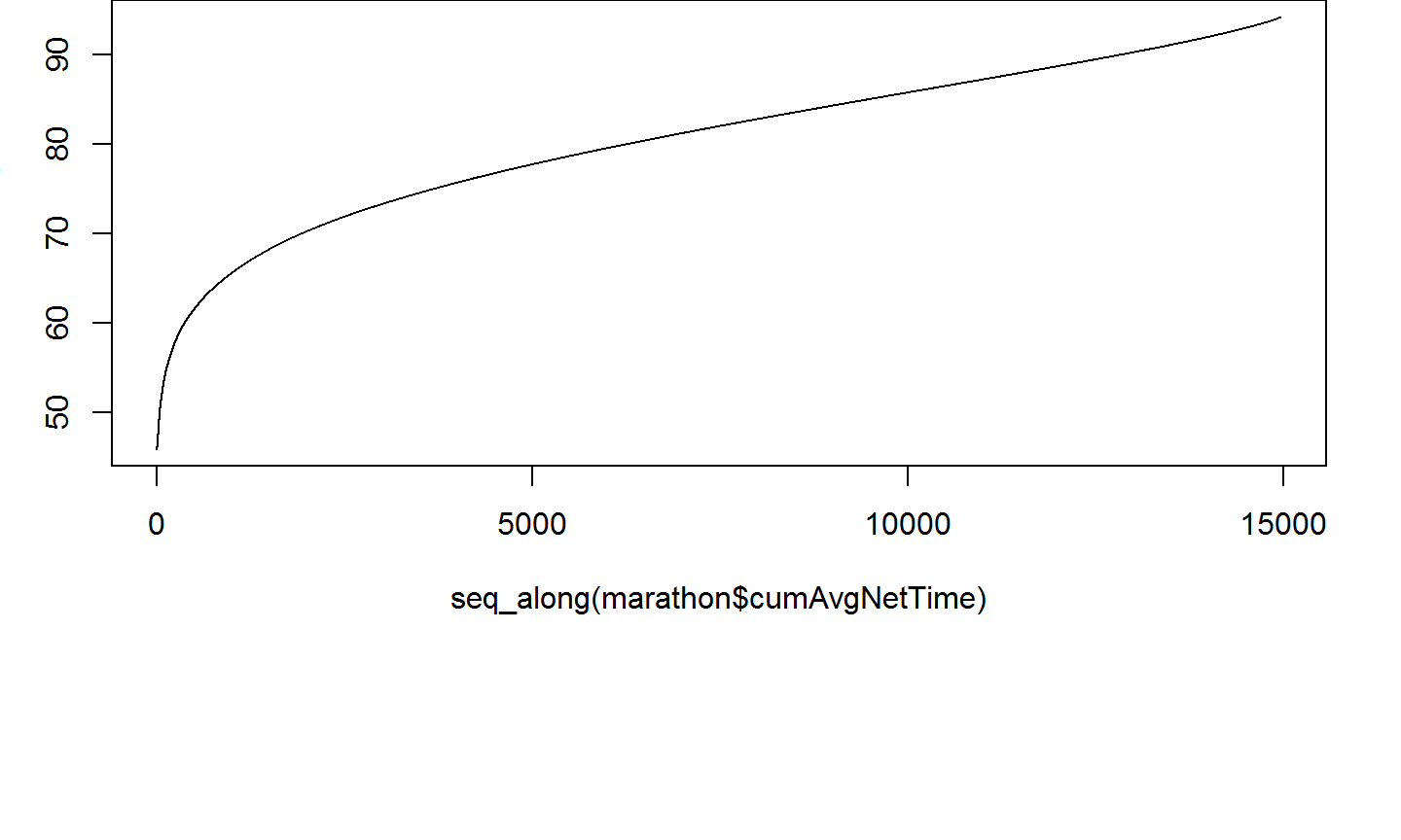
Let's use the cummean function to examine how the average net time changes as each runner finishes the race.

marathon <- marathon %>% mutate(cumAvgNetTime = cummean(netTime))
select(marathon, gender:last, netTime, cumAvgNetTime)

## # A tibble: 14,969 x 5
##   gender first        last        netTime cumAvgNetTime
##   <fct>  <fct>        <fct>         <dbl>         <dbl>
## 1 M      Ridouane     Harroufi       45.9          45.9
## 2 M      Feyisa       Liesa          46.0          46.0
## 3 M      Silas        Sang           46.0          46.0
## 4 M      Karim        El Mabchour    46            46.0
## 5 M      Stephen      Chemlany       46.1          46.0
## 6 M      Cosmas Koech Kimuati        46.1          46.0
## 7 M      Philemon     Terer          46.5          46.1
## 8 M      Samuel       Ndereba        47.0          46.2
## # ... with 1.496e+04 more rows

If you thought that summarizing groups of values and creating complex new variables effortlessly was a powerful set of features, allow me to introduce the do function.

The do function allows you to apply arbitrary functions to the groups of values you have defined.

And by arbitrary, I mean arbitrary. You are not limited to applying functions that return a single values, or exactly n values. You can apply functions that return literally any type of objects.

Allow me to demonstrate by running a linear regression, predicting a runner's net time from their age, on the male and female runners separately.

marathon_lm <- marathon %>% group_by(gender) %>%
  do(time_by_age = lm(netTime~age, data = .))
marathon_lm

## Source: local data frame [2 x 2]
## Groups: <by row>
## 
## # A tibble: 2 x 2
##   gender time_by_age
## * <fct>  <list>     
## 1 F      <S3: lm>   
## 2 M      <S3: lm>

This is possible because data frames may have lists as columns (because data frames are secretely lists!) and lists can hold any type of object.

class(marathon_lm)

## [1] "rowwise_df" "tbl_df"     "tbl"        "data.frame"

class(marathon_lm$time_by_age)

## [1] "list"

class(marathon_lm$time_by_age[[1]])

## [1] "lm"

While do is to summarise as a lightsaber is to a butterknife, great power comes with great responsibility. Working with these special list columns requires both a good understanding of lists, as well as the class of objects you've stored in the list.

So, don't use do when you don't necessarily need its power.

1. Make a new column called division_place that gives a runners place within their own age division (given by the div variable)
   • Hint: There is more than one way to do this (See ?dplyr::ranking for possibilities), but using explicit sorting and the n() function will help you with problem 2.
2. Use the data in the lag_time column we made earlier to make a new variable which shows how much time elapsed between the first place finisher and each remaining runner's finish (e.g., it should tell you how much time passed between the first place finisher and the second place finisher, and the first place finisher and the third place finisher, etc.).
   • Hint: Use one of the cumulative aggregation functions we talked about.

Bonus points for doing this with 1 or fewer variable assignments (i.e., doing it in a single pipeline with %>%).

dplyr provides the cumany and cumall functions, which perform element-wise && and || operations on vectors.

cumall traverses the vector and returns TRUE for each element, until it encounters an element that does not meet the specified criteria. All remaining elements in its output will be FALSE.

Here, cumall searches the vector for "G", and returns TRUE in the first 3 positions, because they are all "G". But after it hits "A" in the fourth position, it returns FALSE for each remaining element.

x <- c("G","G","G","A","G","T","T","C")
cumall(x == "G") # Same as x[1]=="G", x[1]=="G" && x[2]=="G", etc.

## [1]  TRUE  TRUE  TRUE FALSE FALSE FALSE FALSE FALSE

You can think of the cumall function as answering the question "Have all the elements in the vector up to this point met the criteria?"

The cumany function traverses the vector and returns FALSE for each element until it encounters an element that meets the specified criteria. All remaining elements in its output will be TRUE.

x <- c("G","G","G","A","G","T","T","C")
cumany(x == "A")# Same as x[1]=="A", x[1]=="A" || x[3]=="A", etc.

## [1] FALSE FALSE FALSE  TRUE  TRUE  TRUE  TRUE  TRUE

You can think of the cumall function as answering the question "Have any of the elements in the vector up to this point met the criteria?"

These cumulative logical tests can be especially useful for filtering entire groups of observations.

Here we'll use the cumany function to filter the rows of runners who finished after the fastest female runner.

The slice function is used to remove the first row after filtering, so the results don't include the row for the fastest female runner.

marathon %>% filter(cumany(gender == "F")) %>% slice(-1)

## # A tibble: 14,929 x 16
##     age gender first   last  city  state country div   place  time netTime
##   <int> <fct>  <fct>   <fct> <fct> <fct> <fct>   <fct> <int> <dbl>   <dbl>
## 1    29 M      Sam     Blas~ N Po~ MD    USA     25-29    40  53.8    53.8
## 2    21 F      Belian~ Gebre Ethi~ NR    ETH     20-24     2  53.9    53.9
## 3    22 F      Teyba   Naser Ethi~ NR    ETH     20-24     3  54.0    54.0
## 4    24 M      Dylan   Keith Arli~ VA    USA     20-24    41  54.1    54.0
## 5    26 M      Carlos  Renj~ Colu~ MD    USA     25-29    42  54.2    54.1
## 6    25 M      Patrick Murr~ Wash~ DC    USA     25-29    43  54.2    54.2
## 7    37 M      Randy   McDe~ Alex~ VA    USA     35-39    44  54.4    54.3
## 8    19 F      Abebu   Gelan Ethi~ NR    ETH     19-       4  54.4    54.4
## # ... with 1.492e+04 more rows, and 5 more variables: waitTime <dbl>,
## #   quintile <int>, pBelow <dbl>, lag_time <dbl>, cumAvgNetTime <dbl>