- Subsetting is the process of slicing a smaller chunk out of a larger data structure
- Basic syntax template is
DataStructure[IndexVector] - the
IndexVectorcan be a numeric or logical vector - Logical testing uses relational operators like
<and==and logical operators (e.g.,&&and||) to test which elements in our data structure meet specific requirements
2018-05-04
Recall…
Higher Dimensional Structures
Now we'll learn how to index data structures with more than one dimension.
- Recall that Matrices and Data Frames have both rows and columns, making them a 2D data structure
This means when we index them, we must specify which rows we would like to take out in our subset, as well as which columns
Lists are technically 1D vectors, but they have tricky differences from atomic vectors, so we'll save them until the end.
Indexing Matrices
To index a matrix, all that is required is to have two vectors inside our square brackets, separated from each other by a comma.
The template is: OurBigMatrix[rowIndex, columnIndex]
Like with vectors, the index vectors can be either:
- numeric vectors specifying the position of the rows/columns we want to access
- logical vectors specifying for each column and row whether we want to access it (
TRUE) or ignore it (FALSE)
Matrix Examples
Create a small matrix & index it with numeric vectors:
dummy <- matrix(6:1, nrow = 2)
dummy
##      [,1] [,2] [,3]
## [1,]    6    4    2
## [2,]    5    3    1
dummy[1,2:3] # Row 1, Column 2 and 3. Output is a vector!
## [1] 4 2
dummy[1:2,2:3] # Row 1 and 2, Column 2 and 3. Output is a matrix.
##      [,1] [,2]
## [1,]    4    2
## [2,]    3    1
Matrix Examples
If you want to select all of one dimension, (e.g., keep all rows or all columns) but index the other dimension, provide the separating comma as usual, but don't give any indexing vector for the dimension you want to stay 100% intact.
dummy[1,] # First Row, all columns
## [1] 6 4 2
dummy[1,1:3] # Same as previous
## [1] 6 4 2
dummy[,2] # All rows, second columns
## [1] 4 3
dummy[1:2,2] # Same as previous
## [1] 4 3
Logicals & 2D structures
We can apply our relational operators to entire matrices in the same manner as vectors. The resulting logical matrix has the same dimensions as the one we apply the test to.
dummy < 4 # 2 x 3
##       [,1]  [,2] [,3]
## [1,] FALSE FALSE TRUE
## [2,] FALSE  TRUE TRUE
dummy >=3 & dummy <= 5 # also 2 x 3
##       [,1] [,2]  [,3]
## [1,] FALSE TRUE FALSE
## [2,]  TRUE TRUE FALSE
Logicals & 2D structures
We can also apply logical testing and logical indexing to specific dimensions of a matrix.
This example here keeps all the columns of the matrix with a sum less than 8.
colSums(dummy) # colSums() adds up each column
## [1] 11 7 3
colSums(dummy) < 8 # Does each column sum to less than 8?
## [1] FALSE TRUE TRUE
dummy[,colSums(dummy) < 8] # Select columns with a sum less than 8
##      [,1] [,2]
## [1,]    4    2
## [2,]    3    1
Logicals & 2D structures
This example keeps all the rows of the matrix where the value in the first column is greater than 5.
dummy[,1]
## [1] 6 5
dummy[,1] > 5
## [1] TRUE FALSE
dummy[dummy[,1] > 5,] # R drops dimensions by default!
## [1] 6 4 2
dummy[dummy[,1] > 5, ,drop=FALSE] # drop=FALSE preserves dimensions!
##      [,1] [,2] [,3]
## [1,]    6    4    2
Activity
- Create the following matrix \(\left(\begin{array}{cccc} 1 & 4 & 7 \\ 2 & 5 & 8 \\ 3 & 6 & 9 \end{array}\right)\)
- Subset the value from the first row and second column
- Subset the the first and the third column
- Subset the columns that have a mean of more than 4 (Hint: apply the
colMeansfunction to the matrix)
Data Frames
To learn about data frames, we're going to use several data frames that come built-in with R as part of the datasets package. Try typing InsectSprays, iris, airquality and mtcars into the console to be sure they are loaded and available to you.
Since they are included as part of a package, you will not see them listed in your environment pane.
Data Frames
- The
[row,column]indexing style used with matrices also applies to data frames - Data Frames also support a powerful name-based set of indexing operations
- Indexing based on the name you've assigned to a row or column is almost always better, because that name is unlikely to change, while the row or column number is very likely to get changed
- It's also much easier to remember the name of something than remember its position in a data frame
Data Frames
We have previously seen examples of subsetting a single column from a data frame using that columns name, and the $ operator.
mtcars$mpg
##  [1] 21.0 21.0 22.8 21.4 18.7 18.1 14.3 24.4 22.8 19.2 17.8 16.4 17.3 15.2
## [15] 10.4 10.4 14.7 32.4 30.4 33.9 21.5 15.5 15.2 13.3 19.2 27.3 26.0 30.4
## [29] 15.8 19.7 15.0 21.4
Data Frames
To subset multiple columns, we need to use [row,column] style indexing (not the $).
But we're not forced to use numeric vectors just because we're using the [ operator. We can select multiple columns by their names using a character vector that has the names of our desired columns as its elements.
mtcars[,c("mpg","disp","gear")] # need as well as the quotes here
##                      mpg  disp gear
## Mazda RX4           21.0 160.0    4
## Mazda RX4 Wag       21.0 160.0    4
## Datsun 710          22.8 108.0    4
## Hornet 4 Drive      21.4 258.0    3
## Hornet Sportabout   18.7 360.0    3
##  [ reached getOption("max.print") -- omitted 27 rows ]
Data Frames
One of the most common subsetting tasks with a data frame (or matrix) is the need to select values in one column where the values in another column meet a certain criteria.
- You want to select all the values in the column holding reaction times where participants were incorrect
- You want to select values in the column holding the value of a companies net worth for companies founded in the last 5 years
- Infinitely more…
There are 2 syntactic approaches to this, both of which use relational operators & logical indexing.
Method 1: Index the data frame itself
We will use the [row,column] method to pick out the values of the count column in InsectSprays where spray A was used.
- First, we will build up a logical vector to index the correct rows by testing where the spray column has value 'A'
InsectSprays$spray
##  [1] A A A A A A A A A A A A B B B B B B B B B B B B C C C C C C
##  [ reached getOption("max.print") -- omitted 42 entries ]
## Levels: A B C D E F
InsectSprays$spray=="A"
##  [1]  TRUE  TRUE  TRUE  TRUE  TRUE  TRUE  TRUE  TRUE  TRUE  TRUE  TRUE
## [12]  TRUE FALSE FALSE FALSE FALSE FALSE FALSE FALSE FALSE FALSE FALSE
## [23] FALSE FALSE FALSE FALSE FALSE FALSE FALSE FALSE
##  [ reached getOption("max.print") -- omitted 42 entries ]
Method 1: Index the data frame itself
- Next, we combine this with a character vector of the column names we're interested in, and put it inside our
[]brackets
InsectSprays[InsectSprays$spray=="A",'count']
## [1] 10 7 20 14 14 12 10 23 17 20 14 13
- If we leave the column vector out, this statement will return a data frame. Can you guess how many unique values will be in the spray column in this case?
Method 2: Index a vector from the data frame
- Now, we will use the
$operator to subset thecountcolumn from theInsectSpraysdata frame - Then, index this vector with the logical vector resulting from a relational test
InsectSprays$count[InsectSprays$spray=="A"] # Same result as before
## [1] 10 7 20 14 14 12 10 23 17 20 14 13
InsectSprays[InsectSprays$spray=="A",]$count # Still the same. Can you figure out why ?
## [1] 10 7 20 14 14 12 10 23 17 20 14 13
Method 1 vs Method 2: When to use which method?
- Use Method 1 when you want your final result to be a 2D structure
- e.g., if you want to select multiple columns
InsectSprays[InsectSprays$spray=="A",]
- Use Method 2 if you sincerely, 100% want your results to be a vector, and are only interested in subsetting the values of a single column
- It's also fewer key strokes =)
Errors when indexing by name
If you try to subset a column of a data frame using the $ operator, but the name of the column doesn't exist, R will return `NULL``
InsectSprays$neeeeeeighhhhh
## NULL
But, if you use the [row,column] style of indexing and ask for a column that doesn't exist, you get a right proper error.
InsectSprays[, 'neeeeeeighhhhh']
## Error in `[.data.frame`(InsectSprays, , "neeeeeeighhhhh"): undefined columns selected
Errors when indexing by name
[] brackets, which will throw an "object not found" error.
InsectSprays[, spray]
## Error in `[.data.frame`(InsectSprays, , spray): object 'spray' not found
Activity
Using the iris data frame:
- Subset the first 5 and last 5 rows from the data frame, keeping all the columns in your output
- Subset all the rows in the data from where the species is
versicolor, keeping all the column in your output - What species have a recorded sepal width less than 2.1?
Lists
As we learned previously in the Data Structures and Types lessons, lists are the most abstract data structure, capable of holding heterogeneous data types as well as holding other data structures.
Remember, a list is like a directory on your hard drive:
- You can put anything you want in the same directory
- The directory imposes no relationship between the items it holds
- e.g., items don't share rows or columns
- If you don't give the thing you're storing a name, it will be quite hard to find it later since there is no inherent organization other than order
List example
biglist <- list(training = c(1,3,2,4),
                data = data.frame(trial = 1:4,
                                  average = c(.4,.71,.64,.1)),
                times = matrix(c(2.74,3.44,2.91,.65), nrow = 1),
                name = "Herp McDerpsen")
biglist
## $training
## [1] 1 3 2 4
##
## $data
##   trial average
## 1     1    0.40
## 2     2    0.71
## 3     3    0.64
## 4     4    0.10
## $times
##      [,1] [,2] [,3] [,4]
## [1,] 2.74 3.44 2.91 0.65
##
## $name
## [1] "Herp McDerpsen"
Indexing Lists
- Lists elements can have names, and can be accessed by name, just like the columns of a data frame
- Lists are a 1 dimensional structure, so you index into them like a vector
- i.e., no need for
[row, column]style indexing
- i.e., no need for
- Lists may be indexed "normally", using single square brackets (i.e.,
[]), or "recursively", using double square brackets (i.e.,[[]]).
Double vs Single Square Brackets
Indexing a list with a single [] will return a list. But indexing with [[]] returns the actual object stored in that position
biglist[3] # Normal indexing: returns a list with the chosen element(s)
## $times
##      [,1] [,2] [,3] [,4]
## [1,] 2.74 3.44 2.91 0.65
class(biglist[3])
## [1] "list"
biglist[[3]] # Recursive indexing: returns the matrix held in element 3
##      [,1] [,2] [,3] [,4]
## [1,] 2.74 3.44 2.91 0.65
class(biglist[[3]])
## [1] "matrix"
Indexing lists by name
biglist$data # Returns a data frame
##   trial average
## 1     1    0.40
## 2     2    0.71
## 3     3    0.64
## 4     4    0.10
identical(biglist$data, biglist[["data"]]) # $ and [[]] both select single elements
## [1] TRUE
biglist[c("training","name")] # Returns a list of 2
## $training
## [1] 1 3 2 4
##
## $name
## [1] "Herp McDerpsen"
Activity
- Subset the first 3 elements of
biglistby name - Subset the last element of
biglistby position, with the returned value as a list - Extract the character vector stored in the
namefield ofbiglist
Replacing and Removing Values
Replacing and Removing Values
You can use indexing operation on the left hand side of an assignment operation to remove or replace values in your data structure. The basic recipe looks like:
DataObject[LogicalCriteria] <- NewValues
A note of caution: this is an irreversible operation. It would behoove you to make a backup copy of your data structure before altering it, like so:
backup_object <- DataObject
DataObject[LogicalCriteria] <- NewValues
Replacing Values
Lets change the some of pesticide names in the spray column of the InsectSprays data frame to be more informative than just "A", "B", "C", etc.
First, coerce the spray variable from a factor vector into a character vector, for reasons…
InsectSprays$spray <- as.character(InsectSprays$spray)
Then, subset the combination of rows and columns you wish to overwrite, and assign a replacement value to them.
InsectSprays[InsectSprays$spray=='A','spray'] <- "SPRAY_OF_DOOOOM"
InsectSprays[InsectSprays$spray=='B','spray'] <- "fairy_dust"
InsectSprays[c(1,21),]
##    count           spray
## 1     10 SPRAY_OF_DOOOOM
## 21    19      fairy_dust
Removing Columns or List Elements
You can remove single columns from a data frame column or single elements from a list by setting their values to be the NULL object.
backup_iris <- iris
ncol(iris)
## [1] 5
iris$Sepal.Length <- NULL
str(iris)
## 'data.frame':    150 obs. of  4 variables:
##  $ Sepal.Width : num  3.5 3 3.2 3.1 3.6 3.9 3.4 3.4 2.9 3.1 ...
##  $ Petal.Length: num  1.4 1.4 1.3 1.5 1.4 1.7 1.4 1.5 1.4 1.5 ...
##  $ Petal.Width : num  0.2 0.2 0.2 0.2 0.2 0.4 0.3 0.2 0.2 0.1 ...
##  $ Species     : Factor w/ 3 levels "setosa","versicolor",..: 1 1 1 1 1 1 1 1 1 1 ...
Removing Multiple Rows and Columns
Unfortunately, this method of assigning value to be NULL isn't a general solution for all data structures.
When you want to remove rows and columns from matrices and data frame, or individual elements from lists and vectors, is better not to think about deleting at all.
It's more useful to frame the problem in terms of what you want to keep.
Removing Multiple Rows and Columns
For instance, if you think the first 5 rows of a matrix or data frame are useless to you, don't try to delete them in place. Instead, reassign the name of that matrix or data frame to be the result of a subsetting operation that selects only the elements you wish to keep.
iris
##     Sepal.Width Petal.Length Petal.Width    Species
## 1           3.5          1.4         0.2     setosa
## 2           3.0          1.4         0.2     setosa
##  [ reached getOption("max.print") -- omitted 148 rows ]
iris <- iris[6:nrow(iris),]
iris
##     Sepal.Width Petal.Length Petal.Width    Species
## 6           3.9          1.7         0.4     setosa
## 7           3.4          1.4         0.3     setosa
##  [ reached getOption("max.print") -- omitted 143 rows ]
Activity
Use the airquality data frame and do the following:
- Remove the
Windcolumn. - Find the
is.na()function to find and remove rows that are missing observations in theOzonecolumn. - Replace the entries in the
Daycolumn that have value 1 with the character string 'Sunday'.
Advanced Extras
Linear Indexing
Matrices can also be indexed as if they were a 1D structure, like a vector. The figure below shows the mapping between the (row,column) indices and the 'linear indices'. 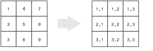
The linear indices start at row 1 of column 1, and travel down the rows of column 1, then continue on in row 1 of column 2, then travel down the rows of column 2, etc…
Linear Indexing
dummy
##      [,1] [,2] [,3]
## [1,]    6    4    2
## [2,]    5    3    1
dummy[2] # Second element
## [1] 5
dummy[5] # Fifth element
## [1] 2
Logicals & 2D structures
This example runs without an error, but the output makes no sense because we are trying to index columns based on the sum of the rows!
dummy[,rowSums(dummy) > 10]
##      [,1] [,2]
## [1,]    6    2
## [2,]    5    1
So it is quite easy to write code that successfully executes, but which produces meaningless output! This is much more insidious than an outright error!
Activity
Try to reason about what R "is doing" in the previous example. Why do we get the output we get?
dummy[,rowSums(dummy) > 10]
##      [,1] [,2]
## [1,]    6    2
## [2,]    5    1
As a hint, try running the code "from the inside out", one logical step at a time.